#### Summary of this post: 

* an overview the motivation behind adversarial autoencoders and how they work * a discussion on whether the adversarial training is necessary in the first place. tl;dr: I think it's an overkill and I propose a simpler method along the lines of kernel moment matching.

#### Adversarial Autoencoders

Again, I recommend everyone interested to read the actual paper, but I'll attempt to give a high level overview the main ideas in the paper. I think the main figure from the paper does a pretty good job explaining how Adversarial Autoencoders are trained:

![](http://www.inference.vc/content/images/2016/01/Screen-Shot-2016-01-08-at-14-48-25.png)

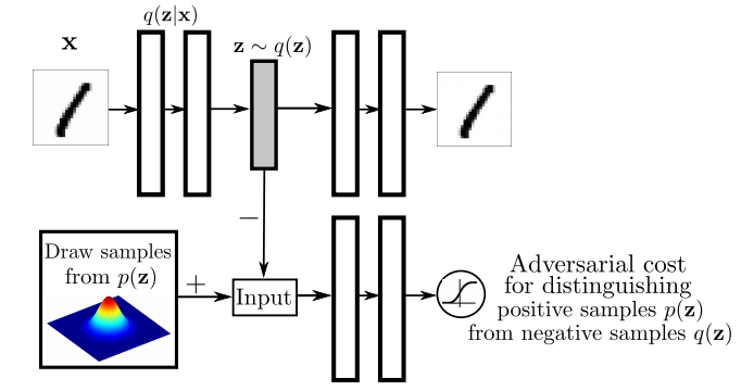
The top part of this image is a probabilistic autoencoder. Given the input $\mathbf{x}$, some latent code $\mathbf{z}$ is generated by sampling from an encoding distribution $q(\mathbf{z}\vert\mathbf{x})$. This distribution is typically modeled as the output a deep neural network. In normal autoencoders this encoder would be deterministic, now we allow it to be probabilistic.

A decoder network is then trained to decode $\mathbf{z}$ and reconstruct the original input $\mathbf{x}$. Of course, reconstruction will not be perfect, but we train the networks to minimise reconstruction error, this is typically just mean squared error.

The reconstruction cost ensures that the encoding process retains information about the input image, but it doesn't enforce anything else about what these latent representations $\mathbf{z}$ should do. In general, their distribution is described as the aggregate posterior $q(\mathbf{z})=\mathbb{E}_\mathbf{x} q(\mathbf{z}\vert\mathbf{x})$. Often, we would like this distribution to match a certain prior $p(\mathbf{z})$. For example. we may want $\mathbf{z}$ to have independent components and Gaussian distributed (nonlinear ICA,PCA). Or we may want to force the latent representations to correspond to discrete class labels, or binary factors. Or we may simply want to ensure there are 'no gaps' in the latent space, and any random $\mathbf{z}$ would lead to a viable sample when squashed through the decoder network.

So there are multiple reasons why one might want to control the aggregate posterior $q(\mathbf{z})$ to match a predefined prior $p(\mathbf{z})$. The authors achieve this by introducing an additional term in the autoencoder loss function, one that measures the divergence between $q$ and $p$. The authors chose to do this via adversarial training: they train a discriminator network that constantly learns to discriminate between real code vectors $\mathbb{z}$ produced by encoding real data, and random code vectors sampled from $p$. If $q$ matches $p$ perfectly, the optimal discriminator network should have a large classification error.

#### Is this an overkill?

My main question about this paper was whether the adversarial cost is really needed here, because I think it's an overkill. Let me explain:

Adversarial training is powerful when all else fails to quantify divergence between complicated, potentially degenerate distributions in high dimensions, such as images or video. Our toolkit for dealing with images is limited, CNNs are the best tool we have, so it makes sense to incorporate them in training generative models for images. GANs - when applied directly to images - are a great idea.

However, here adversarial training is applied to an easier problem: to quantify the divergence between a simple, fixed prior (e.g. Gaussian) and an empirical distribution of latents. The latent space is usually lower-dimensional, distributions better behaved. Therefore, matching to $p(\mathbf{z})$ in latent space should be considerably easier than matching distributions over images.

Adversarial training makes no assumptions about the distributions compared, other than sampling from them. This comes very handy when both $p$ and $q$ are nasty such as in the generative adversarial network scenario: there, $p$ is the distribution of natural images, $q$ is a super complicated, degenerate distribution produced by squashing noise through a deep convnet. The price we pay for this flexibility is this: when $p$ or $q$ are actually easy to work with, adversarial training cannot exploit that, it still has to sample. (it would be interesting to see if expectations over $p(\mathbf{z})$ could be computed analytically). So even though in this work $p$ is as simple as a mixture of ten 2D Gaussians, we need to approximate everything by drawing samples.

#### Other things might work: kernel moment matching

Why can’t one use easier divergences? For example, I think moment matching based on kernel MMD would work brilliantly in this scenario. It would have the following advantages over the adversarial cost.

- closed form expressions: Depending on the choice of the prior $p(\mathbf{z})$ and kernel used in MMD, the expectations over $p$ may be available in closed form, without sampling. So for example if we use a squared exponential kernel and a mixture of Gaussians as $p$, the divergence from $p$ can be precomputed in closed form that is easy to evaluate.

- no nasty inner loop: Adversarial training requires the discriminator network to be reoptimised every time the generative model changes. So we end up with a gradient descent in the inner loop of a gradient descent, which is anything but nice to work with. This is why it takes so long to get it working, the whole thing is pretty unstable. In contrast, to evaluate MMD, the inner loop is not needed. In fact, MMD can also be thought of as the solution to a convex maximisation problem, but via the kernel trick the maximum has a closed form solution.

- the problem is well suited for MMD: because the distributions are smooth, and the space is nice and low-dimensional, MMD might work very well. Kernel-based methods struggle with complicated manifold-like structure of natural images, so I wouldn't expect MMD to be competitive with adversarial training if it is applied directly in the image space. Therefore, I actually prefer generative adversarial networks to generative moment matching networks. However, here we have an easier problem, simpler space, simpler distributions where MMD shines, and adversarial training is just not needed.

The main contribution of [Asynchronous Methods for Deep Reinforcement Learning](https://arxiv.org/pdf/1602.01783v1.pdf) by Mnih et al. is a ligthweight framework for reinforcement learning agents. 

They propose a training procedure which utilizes asynchronous gradient decent updates from multiple agents at once. Instead of training one single agent who interacts with its environment, multiple agents are interacting with their own version of the environment simultaneously.

After a certain amount of timesteps, accumulated gradient updates from an agent are applied to a global model, e.g. a Deep Q-Network. These updates are asynchronous and lock free. 

Effects of training speed and quality are analyzed for various reinforcement learning methods. No replay memory is need to decorrelate successive game states, since all agents are already exploring different game states in real time. Also, on-policy algorithms like actor-critic can be applied.

They show that asynchronous updates have a stabilizing effect on policy and value updates. Also, their best method, an asynchronous variant of actor-critic, surpasses the current state-of-the-art on the Atari domain while training for half the time on a single multi-core CPU instead of a GPU.

Originally posted on my Github [paper-notes](https://github.com/karpathy/paper-notes/blob/master/matching_networks.md) repo.

# Matching Networks for One Shot Learning

By DeepMind crew: **Oriol Vinyals, Charles Blundell, Timothy Lillicrap, Koray Kavukcuoglu, Daan Wierstra**

This is a paper on **one-shot** learning, where we'd like to learn a class based on very few (or indeed, 1) training examples. E.g. it suffices to show a child a single giraffe, not a few hundred thousands before it can recognize more giraffes.

This paper falls into a category of *"duh of course"* kind of paper, something very interesting, powerful, but somehow obvious only in retrospect. I like it.

Suppose you're given a single example of some class and would like to label it in test images.

- **Observation 1**: a standard approach might be to train an Exemplar SVM for this one (or few) examples vs. all the other training examples - i.e. a linear classifier. But this requires optimization.
- **Observation 2:** known non-parameteric alternatives (e.g. k-Nearest Neighbor) don't suffer from this problem. E.g. I could immediately use a Nearest Neighbor to classify the new class without having to do any optimization whatsoever. However, NN is gross because it depends on an (arbitrarily-chosen) metric, e.g. L2 distance. Ew.
- **Core idea**: lets train a fully end-to-end nearest neighbor classifer!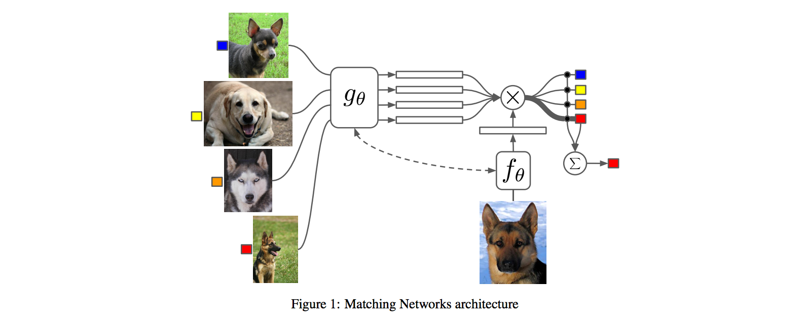![Screen Shot 2016-08-07 at 10.08.44 PM](https://raw.githubusercontent.com/karpathy/paper-notes/master/img/matching_networks/Screen%20Shot%202016-08-07%20at%2010.08.44%20PM.png)

## The training protocol

As the authors amusingly point out in the conclusion (and this is the *duh of course* part), *"one-shot learning is much easier if you train the network to do one-shot learning"*. Therefore, we want the test-time protocol (given N novel classes with only k examples each (e.g. k = 1 or 5), predict new instances to one of N classes) to exactly match the training time protocol.

To create each "episode" of training from a dataset of examples then:

1. Sample a task T from the training data, e.g. select 5 labels, and up to 5 examples per label (i.e. 5-25 examples).
2. To form one episode sample a label set L (e.g. {cats, dogs}) and then use L to sample the support set S and a batch B of examples to evaluate loss on.

The idea on high level is clear but the writing here is a bit unclear on details, of exactly how the sampling is done.

## The model

I find the paper's model description slightly wordy and unclear, but basically we're building a **differentiable nearest neighbor++**. The output \hat{y} for a test example \hat{x} is computed very similar to what you might see in Nearest Neighbors:![Screen Shot 2016-08-07 at 11.14.26 PM](https://raw.githubusercontent.com/karpathy/paper-notes/master/img/matching_networks/Screen%20Shot%202016-08-07%20at%2011.14.26%20PM.png)
where **a** acts as a kernel, computing the extent to which \hat{x} is similar to a training example x_i, and then the labels from the training examples (y_i) are weight-blended together accordingly. The paper doesn't mention this but I assume for classification y_i would presumbly be one-hot vectors.

Now, we're going to embed both the training examples x_i and the test example \hat{x}, and we'll interpret their inner products (or here a cosine similarity) as the "match", and pass that through a softmax to get normalized mixing weights so they add up to 1. No surprises here, this is quite natural:

![Screen Shot 2016-08-07 at 11.20.29 PM](https://raw.githubusercontent.com/karpathy/paper-notes/master/img/matching_networks/Screen%20Shot%202016-08-07%20at%2011.20.29%20PM.png)
Here **c()** is cosine distance, which I presume is implemented by normalizing the two input vectors to have unit L2 norm and taking a dot product. I assume the authors tried skipping the normalization too and it did worse? Anyway, now all that's left to define is the function **f** (i.e. how do we embed the test example into a vector) and the function **g** (i.e. how do we embed each training example into a vector?).

**Embedding the training examples.** This (the function **g**) is a bidirectional LSTM over the examples:

 ![Screen Shot 2016-08-07 at 11.57.10 PM](https://raw.githubusercontent.com/karpathy/paper-notes/master/img/matching_networks/Screen%20Shot%202016-08-07%20at%2011.57.10%20PM.png)

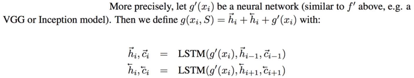
i.e. encoding of i'th example x_i is a function of its "raw" embedding g'(x_i) and the embedding of its friends, communicated through the bidirectional network's hidden states. i.e. each training example is a function of not just itself but all of its friends in the set. This is part of the ++ above, because in a normal nearest neighbor you wouldn't change the representation of an example as a function of the other data points in the training set.

It's odd that the **order** is not mentioned, I assume it's random? This is a bit gross because order matters to a bidirectional LSTM; you'd get different embeddings if you permute the examples. 

**Embedding the test example.** This (the function **f**) is a an LSTM that processes for a fixed amount (K time steps) and at each point also *attends* over the examples in the training set. The encoding is the last hidden state of the LSTM. Again, this way we're allowing the network to change its encoding of the test example as a function of the training examples. Nifty: 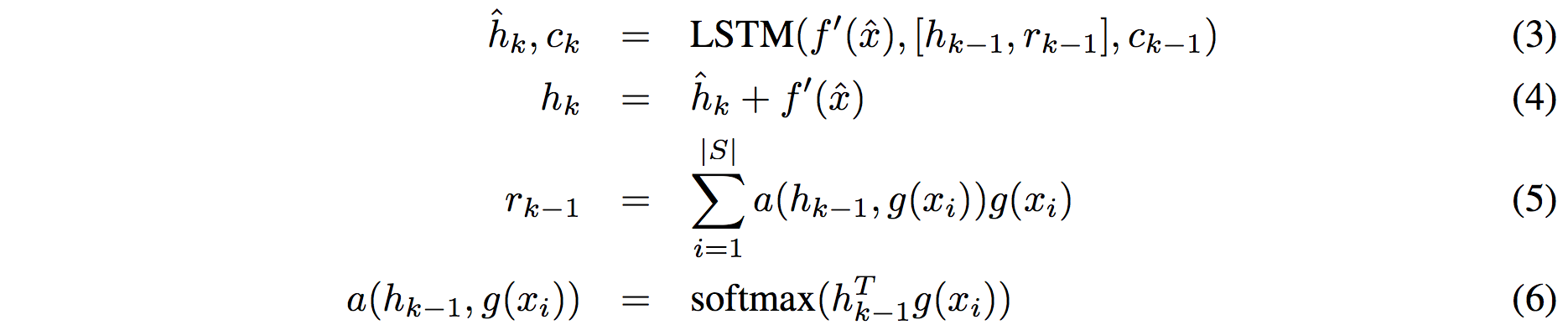![Screen Shot 2016-08-08 at 12.11.15 AM](https://raw.githubusercontent.com/karpathy/paper-notes/master/img/matching_networks/Screen%20Shot%202016-08-08%20at%2012.11.15%20AM.png)

That looks scary at first but it's really just a vanilla LSTM with attention where the input at each time step is constant (f'(\hat{x}), an encoding of the test example all by itself) and the hidden state is a function of previous hidden state but also a concatenated readout vector **r**, which we obtain by attending over the encoded training examples (encoded with **g** from above).

Oh and I assume there is a typo in equation (5), it should say r_k = … without the -1 on LHS. 



## Experiments

**Task**: N-way k-shot learning task. i.e. we're given k (e.g. 1 or 5) labelled examples for N classes that we have not previously trained on and asked to classify new instances into he N classes.

**Baselines:** an "obvious" strategy of using a pretrained ConvNet and doing nearest neighbor based on the codes. An option of finetuning the network on the new examples as well (requires training and careful and strong regularization!).

**MANN** of Santoro et al. [21]: Also a DeepMind paper, a fun NTM-like Meta-Learning approach that is fed a sequence of examples and asked to predict their labels.

**Siamese network** of Koch et al. [11]: A siamese network that takes two examples and predicts whether they are from the same class or not with logistic regression. A test example is labeled with a nearest neighbor: with the class it matches best according to the siamese net (requires iteration over all training examples one by one). Also, this approach is less end-to-end than the one here because it requires the ad-hoc nearest neighbor matching, while here the *exact* end task is optimized for. It's beautiful.



### Omniglot experiments 

### ![Screen Shot 2016-08-08 at 10.21.45 AM](https://github.com/karpathy/paper-notes/raw/master/img/matching_networks/Screen%20Shot%202016-08-08%20at%2010.21.45%20AM.png)

Omniglot of [Lake et al. [14]](http://www.cs.toronto.edu/~rsalakhu/papers/LakeEtAl2015Science.pdf) is a MNIST-like scribbles dataset with 1623 characters with 20 examples each.

Image encoder is a CNN with 4 modules of [3x3 CONV 64 filters, batchnorm, ReLU, 2x2 max pool]. The original image is claimed to be so resized from original 28x28 to 1x1x64, which doesn't make sense because factor of 2 downsampling 4 times is reduction of 16, and 28/16 is a non-integer >1. I'm assuming they use VALID convs?

Results: 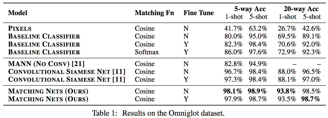![Screen Shot 2016-08-08 at 10.27.46 AM](https://raw.githubusercontent.com/karpathy/paper-notes/master/img/matching_networks/Screen%20Shot%202016-08-08%20at%2010.27.46%20AM.png)

Matching nets do best. Fully Conditional Embeddings (FCE) by which I mean they the "Full Context Embeddings" of Section 2.1.2 instead are not used here, mentioned to not work much better. Finetuning helps a bit on baselines but not with Matching nets (weird).

The comparisons in this table are somewhat confusing:

- I can't find the MANN numbers of 82.8% and 94.9% in their paper [21]; not clear where they come from. E.g. for 5 classes and 5-shot they seem to report 88.4% not 94.9% as seen here. I must be missing something.
- I also can't find the numbers reported here in the Siamese Net [11] paper. As far as I can tell in their Table 2 they report one-shot accuracy, 20-way classification to be 92.0, while here it is listed as 88.1%?
- The results of Lake et al. [14] who proposed Omniglot are also missing from the table. If I'm understanding this correctly they report 95.2% on 1-shot 20-way, while matching nets here show 93.8%, and humans are estimated at 95.5%. That is, the results here appear weaker than those of Lake et al., but one should keep in mind that the method here is significantly more generic and does not make any assumptions about the existence of strokes, etc., and it's a simple, single fully-differentiable blob of neural stuff.

(skipping ImageNet/LM experiments as there are few surprises)

## Conclusions

Good paper, effectively develops a differentiable nearest neighbor trained end-to-end. It's something new, I like it!

A few concerns: 

- A bidirectional LSTMs (not order-invariant compute) is applied over sets of training examples to encode them. The authors don't talk about the order actually used, which presumably is random, or mention this potentially unsatisfying feature. This can be solved by using a recurrent attentional mechanism instead, as the authors are certainly aware of and as has been discussed at length in [ORDER MATTERS: SEQUENCE TO SEQUENCE FOR SETS](https://arxiv.org/abs/1511.06391), where Oriol is also the first author. I wish there was a comment on this point in the paper somewhere.

- The approach also gets quite a bit slower as the number of training examples grow, but once this number is large one would presumable switch over to a parameteric approach.

- It's also potentially concerning that during training the method uses a specific number of examples, e.g. 5-25, so this is the number of that must also be used at test time. What happens if we want the size of our training set to grow online? It appears that we need to retrain the network because the encoder LSTM for the training data is not "used to" seeing inputs of more examples? That is unless you fall back to iteratively subsampling the training data, doing multiple inference passes and averaging, or something like that. If we don't use FCE it can still be that the attention mechanism LSTM can still not be "used to" attending over many more examples, but it's not clear how much this matters. An interesting experiment would be to not use FCE and try to use 100 or 1000 training examples, while only training on up to 25 (with and fithout FCE). Discussion surrounding this point would be interesting.

- Not clear what happened with the Omniglot experiments, with incorrect numbers for [11], [21], and the exclusion of Lake et al. [14] comparison.

- A baseline that is missing would in my opinion also include training of an [Exemplar SVM](https://www.cs.cmu.edu/~tmalisie/projects/iccv11/), which is a much more powerful approach than encode-with-a-cnn-and-nearest-neighbor.

  ​

The [paper](http://vldb.org/pvldb/vol5/p1771_georgelee_vldb2012.pdf) presents Twitter's logging infrastructure, how it evolved from application specific logging to a unified logging infrastructure and how session-sequences are used as a common case optimization for a large class of queries.

## Messaging Infrastructure

Twitter uses **Scribe** as its messaging infrastructure. A Scribe daemon runs on every production server and sends log data to a cluster of dedicated aggregators in the same data center. Scribe itself uses **Zookeeper** to discover the hostname of the aggregator. Each aggregator registers itself with Zookeeper. The Scribe daemon consults Zookeeper to find a live aggregator to which it can send the data. Colocated with the aggregators is the staging Hadoop cluster which merges the per-category stream from all the server daemons and writes the compressed results to HDFS. These logs are then moved into main Hadoop data warehouse and are deposited in per-category, per-hour directory (eg /logs/category/YYYY/MM/DD/HH). Within each directory, the messages are bundled in a small number of large files and are partially ordered by time.

Twitter uses **Thrift** as its data serialization framework, as it supports nested structures, and was already being used elsewhere within Twitter. A system called **Elephant Bird** is used to generate Hadoop record readers and writers for arbitrary thrift messages. Production jobs are written in **Pig(Latin)** and scheduled using **Oink**.

## Application Specific Logging

Initially, all applications defined their own custom formats for logging messages. While it made it easy to develop application logging, it had many downsides as well.

* Inconsistent naming conventions: eg uid vs userId vs user_Id
* Inconsistent semantics associated with each category name causing resource discovery problem.
* Inconsistent format of log messages.

All these issues make it difficult to reconstruct user session activity. 

## Client Events

This is an effort within Twitter to develop a unified logging framework to get rid of all the issues discussed previously. A hierarchical, 6-level schema is imposed on all the events (as described in the table below).



| Component |  Description                       |  Example                                     | 
|-----------|------------------------------------|----------------------------------------------| 
| client    |  client application                |  web, iPhone, android                          | 
| page      |  page or functional grouping       |  home, profile, who_to_follow                  | 
| section   |  tab or stream on a page           |  home, mentions, retweets, searches, suggestions | 
| component |  component object or objects       |  search_box, tweet                            | 
| element   |  UI element within the component   |  button, avatar                               | 
| action    |  actual user or application action |  impression, click, hover                      | 


**Table 1: Hierarchical decomposition of client event names.**

For example, the following event, `web:home:mentions:stream:avatar:profile_click` is logged whenever there is an image profile click on the avatar of a tweet in the mentions timeline for a user on twitter.com (read from right to left).

The alternate design was a tree based model for logging client events. That model allowed for arbitrarily deep event namespace with as fine-grained logging as required. But the client events model was chosen to make the top level aggregate queries easier.

A client event is a Thrift structure that contains the components given in the table below.

| Field           | Description                     | 
|-----------------|---------------------------------| 
| event initiator |  {client, server} × {user, app} | 
| event_name      |  event name                     | 
| user_id         |  user id                        | 
| session_id      |  session id                     | 
| ip              |  user’s IP address              | 
| timestamp       |  timestamp                      | 
| event_details   |  event details                  | 

**Table 2: Definition of a client event.**

The logging infrastructure is unified in two senses: 

* All log messages share a common format with clear semantics.
* All log messages are stored in a single place.

## Session Sequences

A session sequence is a sequence of symbols *S = {s<sub>0</sub>, s<sub>1</sub>, s<sub>2</sub>...s<sub>n</sub>}* such that each symbol is drawn from a finite alphabet *Σ*. A bijective mapping is defined between Σ and universe of event names. Each symbol in Σ is represented by a valid Unicode point (frequent events are assigned shorter code prints) and each session sequence becomes a valid Unicode string. Once all logs have been imported to the main database, a histogram of event counts is created and is used to map event names to Unicode code points. The counts and samples of each event type are stored in a known location in HDFS. Session sequences are reconstructed from the raw client event logs via a *group-by* on *user_id* and *session_id*. Session sequences are materialized as it is difficult to work with raw client event logs for following reasons:
* A lot of brute force scans.
* Large group-by operations needed to reconstruct user session.

#### Alternate Designs Considered
* Reorganize complete Thrift messages by reconstructing user sessions - This solves the second problem but not the first.
* Use a columnar storage format - This addresses the first issue but it just reduces the time taken by mappers and not the number of mappers itself.

The materialized session sequences are much smaller than raw client event logs (around 50 times smaller) and address both the issues.

## Client Event Catalog

To enhance the accessibility of the client event logs, an automatically generated event data log is used along with a browsing interface to allow users to browse, search and access sample entries for the various client events. (These sample entries are the same entries that were mentioned in the previous section. The catalog is rebuilt every day and is always up to date.

## Applications

Client Event Logs and Session Sequences are used in following applications:

* Summary Statistics - Session sequences are used to compute various statistics about sessions.
* Event Counting - Used to understand what feature of users take advantage of a particular feature.
* Funnel Analytics - Used to focus on user attention in a multi-step process like signup process.
* User Modeling - Used to identify "interesting" user behavior. N-gram models (from NLP domain) can be extended to measure how important temporal signals are by modeling user behavior on the basis of last n actions. The paper also mentions the possibility of extracting "activity collocations" based on the notion of collocations.


## Possible Extensions

Session sequences are limited in the sense that they capture only event name and exclude other details. The solution adopted by Twitter is to use a generic indexing infrastructure that integrates with Hadoop at the level of InputFormats. The indexes reside with the data making it easier to reindex the data. An alternative would have been to use **Trojan layouts** which members indexing in HDFS block header but this means that indexing would require the data to be rewritten. Another possible extension would be to leverage more analogies from the field of Natural Language Processing. This would include the use of automatic grammar induction techniques to learn hierarchical decomposition of user activity. Another area of exploration is around leveraging advanced visualization techniques for exploring sessions and mapping interesting behavioral patterns into distinct visual patterns that can be easily recognized.

#### Introduction

* Method to visualize high-dimensional data points in 2/3 dimensional space.
* Data visualization techniques like Chernoff faces and graph approaches just provide a representation and not an interpretation.
* Dimensionality reduction techniques fail to retain both local and global structure of the data simultaneously. For example, PCA and MDS are linear techniques and fail on data lying on a non-linear manifold.
* t-SNE approach converts data into a matrix of pairwise similarities and visualizes this matrix.
* Based on SNE (Stochastic Neighbor Embedding)
* [Link to paper](http://jmlr.csail.mit.edu/papers/volume9/vandermaaten08a/vandermaaten08a.pdf)

#### SNE

* Given a set of datapoints $x_1, x_2, ...x_n, p_{i|j}$ is the probability that $x_i$ would pick $x_j$ as its neighbor if neighbors were picked in proportion to their probability density under a Gaussian centered at $x_i$. Calculation of $\sigma_i$ is described later.
* Similarly, define $q_{i|j}$ as conditional probability corresponding to low-dimensional representations of $y_i$ and $y_j$ (corresponding to $x_i$ and $x_j$). The variance of Gaussian in this case is set to be $1/\sqrt{2}$
* Argument is that if $y_i$ and $y_j$ captures the similarity between $x_i$ and $x_j$, $p_{i|j}$ and $q_{i|j}$ should be equal. So objective function to be minimized is Kullback-Leibler (KL) Divergence measure for $P_i$ and $Q_i$, where $P_i$ ($Q_i$) represent conditional probability distribution given $x_i$ ($y_i$)
* Since KL Divergence is not symmetric, the objective function focuses on retaining the local structure.
* Users specify a value called perplexity (measure of effective number of neighbors). A binary search is performed to find $\sigma_i$ which produces the $P_i$ having same perplexity as specified by the user.
* Gradient Descent (with momentum) is used to minimize objective function and Gaussian noise is added in early stages to perform simulated annealing.

#### t-SNE (t-Distributed SNE)

##### Symmetric SNE

* A single KL Divergence between P (joint probability distribution in high-dimensional space) and Q (joint probability distribution in low-dimensional space) is minimized.
* Symmetric because $p_{i|j} = p_{j|i}$ and $q_{i|j} = q_{j|i}$
* More robust to outliers and has a simpler gradient expression.

##### Crowding Problem

* When we model a high-dimensional dataset in 2 (or 3) dimensions, it is difficult to segregate the nearby datapoints from moderately distant datapoints and gaps can not form between natural clusters.
* One way around this problem is to use UNI-SNE but optimization of the cost function, in that case, is difficult.

##### t-SNE

* Instead of Gaussian, use a heavy-tailed distribution (like Student-t distribution) to convert distances into probability scores in low dimensions. This way moderate distance in high-dimensional space can be modeled by larger distance in low-dimensional space.
* Student-t distribution is an infinite mixture of Gaussians and density for a point under this distribution can be computed very fast. 
* The cost function is easy to optimize.

##### Optimization Tricks

###### Early Compression

* At the start of optimization, force the datapoints (in low-dimensional space) to stay close together so that datapoints can easily move from one cluster to another. 
* Implemented an L2-penalty term proportional to the sum of the squared distance of datapoints from the origin.

###### Early Exaggeration

* Scale all the $p_{i|j}$'s so that large $q_{i|j}$*'s are obtained with the effect that natural clusters in the data form tight, widely separated clusters as a lot of empty space is created in the low-dimensional space.

##### t-SNE on large datasets

* Space and time complexity is quadratic in the number of datapoints so infeasible to apply on large datasets.
* Select a random subset of points (called landmark points) to display.
* for each landmark point, define a random walk starting at a landmark point and terminating at any other landmark point.
* $p_{i|j}$ is defined as fraction of random walks starting at $x_i$ and finishing at $x_j$ (both these points are landmark points). This way, $p_{i|j}$ is not sensitive to "short-circuits" in the graph (due to noisy data points).

#### Advantages of t-SNE

* Gaussian kernel employed by t-SNE (in high-dimensional) defines a soft border between the local and global structure of the data.
* Both nearby and distant pair of datapoints get equal importance in modeling the low-dimensional coordinates.
* The local neighborhood size of each datapoint is determined on the basis of the local density of the data.
* Random walk version of t-SNE takes care of "short-circuit" problem.

#### Limitations of t-SNE

* It is unclear t-SNE would perform on general **Dimensionality Reduction** for more than 3 dimensions. For such higher (than 3) dimensions, Student-t distribution with more degrees of freedom should be more appropriate.
* t-SNE reduces the dimensionality of data mainly based on local properties of the data which means it would fail in data which has intrinsically high dimensional structure (**curse of dimensionality**).
* The cost function for t-SNE is not convex requiring several optimization parameters to be chosen which would affect the constructed solution.