* The paper describes a method to separate content and style from each other in an image.
  * The style can then be transfered to a new image.
  * Examples:
    * Let a photograph look like a painting of van Gogh.
    * Improve a dark beach photo by taking the style from a sunny beach photo.

### How
  * They use the pretrained 19-layer VGG net as their base network.
  * They assume that two images are provided: One with the *content*, one with the desired *style*.
  * They feed the content image through the VGG net and extract the activations of the last convolutional layer. These activations are called the *content representation*.
  * They feed the style image through the VGG net and extract the activations of all convolutional layers. They transform each layer to a *Gram Matrix* representation. These Gram Matrices are called the *style representation*.
  * How to calculate a *Gram Matrix*:
    * Take the activations of a layer. That layer will contain some convolution filters (e.g. 128), each one having its own activations.
    * Convert each filter's activations to a (1-dimensional) vector.
    * Pick all pairs of filters. Calculate the scalar product of both filter's vectors.
    * Add the scalar product result as an entry to a matrix of size `#filters x #filters` (e.g. 128x128).
    * Repeat that for every pair to get the Gram Matrix.
    * The Gram Matrix roughly represents the *texture* of the image.
  * Now you have the content representation (activations of a layer) and the style representation (Gram Matrices).
  * Create a new image of the size of the content image. Fill it with random white noise.
  * Feed that image through VGG to get its content representation and style representation. (This step will be repeated many times during the image creation.)
  * Make changes to the new image using gradient descent to optimize a loss function.
    * The loss function has two components:
      * The mean squared error between the new image's content representation and the previously extracted content representation.
      * The mean squared error between the new image's style representation and the previously extracted style representation.
    * Add up both components to get the total loss.
    * Give both components a weight to alter for more/less style matching (at the expense of content matching).


![Examples](https://raw.githubusercontent.com/aleju/papers/master/neural-nets/images/A_Neural_Algorithm_for_Artistic_Style__examples.jpg?raw=true "Examples")

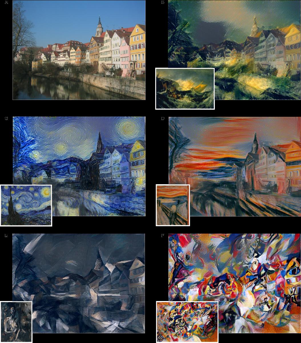
*One example input image with different styles added to it.*

-------------------------

### Rough chapter-wise notes

* Page 1
  * A painted image can be decomposed in its content and its artistic style.
  * Here they use a neural network to separate content and style from each other (and to apply that style to an existing image).

* Page 2
  * Representations get more abstract as you go deeper in networks, hence they should more resemble the actual content (as opposed to the artistic style).
  * They call the feature responses in higher layers *content representation*.
  * To capture style information, they use a method that was originally designed to capture texture information.
  * They somehow build a feature space on top of the existing one, that is somehow dependent on correlations of features. That leads to a "stationary" (?) and multi-scale representation of the style.

* Page 3
  * They use VGG as their base CNN.

* Page 4
  * Based on the extracted style features, they can generate a new image, which has equal activations in these style features.
  * The new image should match the style (texture, color, localized structures) of the artistic image.
  * The style features become more and more abtstract with higher layers. They call that multi-scale the *style representation*.
  * The key contribution of the paper is a method to separate style and content representation from each other.
  * These representations can then be used to change the style of an existing image (by changing it so that its content representation stays the same, but its style representation matches the artwork).

* Page 6
  * The generated images look most appealing if all features from the style representation are used. (The lower layers tend to reflect small features, the higher layers tend to reflect larger features.)
  * Content and style can't be separated perfectly.
  * Their loss function has two terms, one for content matching and one for style matching.
  * The terms can be increased/decreased to match content or style more.

* Page 8
  * Previous techniques work only on limited or simple domains or used non-parametric approaches (see non-photorealistic rendering).
  * Previously neural networks have been used to classify the time period of paintings (based on their style).
  * They argue that separating content from style might be useful and many other domains (other than transfering style of paintings to images).

* Page 9
  * The style representation is gathered by measuring correlations between activations of neurons.
  * They argue that this is somehow similar to what "complex cells" in the primary visual system (V1) do.
  * They note that deep convnets seem to automatically learn to separate content from style, probably because it is helpful for style-invariant classification.

* Page 9, Methods
  * They use the 19 layer VGG net as their basis.
  * They use only its convolutional layers, not the linear ones.
  * They use average pooling instead of max pooling, as that produced slightly better results.

* Page 10, Methods
  * The information about the image that is contained in layers can be visualized. To do that, extract the features of a layer as the labels, then start with a white noise image and change it via gradient descent until the generated features have minimal distance (MSE) to the extracted features.
  * The build a style representation by calculating Gram Matrices for each layer.

* Page 11, Methods
  * The Gram Matrix is generated in the following way:
    * Convert each filter of a convolutional layer to a 1-dimensional vector.
    * For a pair of filters i, j calculate the value in the Gram Matrix by calculating the scalar product of the two vectors of the filters.
    * Do that for every pair of filters, generating a matrix of size #filters x #filters. That is the Gram Matrix.
  * Again, a white noise image can be changed with gradient descent to match the style of a given image (i.e. minimize MSE between two Gram Matrices).
  * That can be extended to match the style of several layers by measuring the MSE of the Gram Matrices of each layer and giving each layer a weighting.

* Page 12, Methods
  * To transfer the style of a painting to an existing image, proceed as follows:
    * Start with a white noise image.
    * Optimize that image with gradient descent so that it minimizes both the content loss (relative to the image) and the style loss (relative to the painting).
    * Each distance (content, style) can be weighted to have more or less influence on the loss function.

This paper describes how rank pooling, a very recent approach for pooling representations organized in a sequence $\\{{\bf v}_t\\}_{t=1}^T$, can be used in an end-to-end trained neural network architecture.

Rank pooling is an alternative to average and max pooling for sequences, but with the distinctive advantage of maintaining some order information from the sequence. Rank pooling first solves a regularized (linear) support vector regression (SVR) problem where the inputs are the vector representations ${\bf v}_t$ in the sequence and the target is the corresponding index $t$ of that representation in the sequence (see Equation 5). The output of rank pooling is then simply the linear regression parameters $\bf{u}$ learned for that sequence. Because of the way ${\bf u}$ is trained, we can see that ${\bf u}$ will capture order information, as successful training would imply that ${\bf u}^\top {\bf v}_t < {\bf u}^\top {\bf v}_{t'} $ if $t < t'$. See [this paper](https://www.robots.ox.ac.uk/~vgg/rg/papers/videoDarwin.pdf) for more on rank pooling.

While previous work has focused on using rank pooling on hand-designed and fixed representations, this paper proposes to use ConvNet features (pre-trained on ImageNet) for the representation and backpropagate through rank pooling to fine-tune the ConvNet features. Since the output of rank pooling corresponds to an argmin operation, passing gradients through this operation is not as straightforward as for average or max pooling. However, it turns out that if the objective being minimized (in our case regularized SVR) is twice differentiable, gradients with respect to its argmin can be computed (see Lemmas 1 and 2). The authors derive the gradient for rank pooling (Equation 21). Finally, since its gradient requires inverting a matrix (corresponding to a hessian), the authors propose to either use an efficient procedure for computing it by exploiting properties of sums of rank-one matrices (see Lemma 3) or to simply use an approximation based on using a diagonal hessian.

In experiments on two small scale video activity recognition datasets (UCF-Sports and Hollywood2), the authors show that fine-tuning the ConvNet features significantly improves the performance of rank pooling and makes it superior to max and average pooling.

**My two cents**

This paper was eye opening for me, first because I did not realize that one could backpropagate through an operation corresponding to an argmin that doesn't have a closed form solution (though apparently this paper isn't the first to make that observation). Moreover, I did not know about rank pooling, which itself is a really thought provoking approach to pooling representations in a way that preserves some organizational information about the original representations.

I wonder how sensitive the results are to the value of the regularization constant of the SVR problem. The authors mention some theoretical guaranties on the stability of the solution found by SVR in general, but intuitively I would expect that the regularization constant would play a large role in the stability.

I'll be looking forward to any future attempts to increase the speed of rank pooling (or any similar method). Indeed, as the authors mention, it is currently too slow to be used on the larger video datasets that are currently available. 

Code for computing rank pooling (though not for computing its gradients) seems to be available [here](https://bitbucket.org/bfernando/videodarwin).

(See also a more thorough summary in [a LaTeX PDF][1].)

This paper has some nice clear theory which bridges maximum likelihood (supervised) learning and standard reinforcement learning. It focuses on *structured prediction* tasks, where we want to learn to predict $p_\theta(y \mid x)$ where $y$ is some object with complex internal structure.

We can agree on some deficiencies of maximum likelihood learning:

- ML training fails to assign **partial credit**. Models are trained to maximize the likelihood of the ground-truth outputs in the dataset, and all other outputs are equally wrong. This is an increasingly important problem as the space of possible solutions grows.
- ML training is potentially disconnected from **downstream task reward**. In machine translation, we usually want to optimize relatively complex metrics like BLEU or TER. Since these metrics are non-differentiable, we have to settle for optimizing proxy losses that we hope are related to the metric of interest.

Reinforcement learning offers an attractive alternative in theory. RL algorithms are designed to optimize non-differentiable (even stochastic) reward functions, which sounds like just what we want. But RL algorithms have their own problems with this sort of structured output space:

- Standard RL algorithms rely on samples from the model we are learning, $p_\theta(y \mid x)$. This becomes intractable when our output space is very complex (e.g. 80-token sequences where each word is drawn from a vocabulary of 80,000 words).
- The reward spaces for problems of interest are extremely sparse. Our metrics will assign 0 reward to most of the 80^80K possible outputs in the translation problem in the paper.
- Vanilla RL doesn't take into account the ground-truth outputs available to us in structured prediction.

This paper designs a solution which combines supervised learning with a reinforcement learning-inspired smoothing method. Concretely, the authors design an **exponentiated payoff distribution** $q(y \mid y^*; \tau)$ which assigns high mass to high-reward outputs $y$ and low mass elsewhere. This distribution is used to effectively smooth the loss function established by the ground-truth outputs in the supervised data. We end up optimizing the following objective:

$$\mathcal L_\text{RML} = - \mathbb E_{x, y^* \sim \mathcal D}\left[ \sum_y q(y \mid y^*; \tau) \log p_\theta(y \mid x) \right]$$

This optimization depends on samples from our dataset $\mathcal D$ and, more importantly, the stationary payoff distribution $q$. This contrasts strongly with standard RL training, where the objective depends on samples from the non-stationary model distribution $p_\theta$. To make that clear, we can rewrite the above with another expectation:

$$\mathcal L_\text{RML} = - \mathbb E_{x, y^* \sim \mathcal D, y \sim q(y \mid y^*; \tau)}\left[ \log p_\theta(y \mid x) \right]$$

### Model details

If you're interested in the low-level details, I wrote up the gist of the math in [this PDF][1].

### Analysis

#### Relationship to label smoothing

This training approach is mathematically equivalent to label smoothing, applied here to structured output problems. In next-word prediction language modeling, a popular trick involves smoothing the target distributions by combining the ground-truth output with some simple base model, e.g. a unigram word frequency distribution. (This just means we take a weighted sum of the one-hot vector from our supervised data and a normalized frequency vector calculated on some corpus.) Mathematically, the cross entropy with label smoothing is

$$\mathcal L_\text{ML-smooth} = - \mathbb E_{x, y^* \sim \mathcal D} \left[ \sum_y p_\text{smooth}(y; y^*) \log p_\theta(y \mid x) \right]$$

(The equation above leaves out a constant entropy term.)

The gradient of this objective looks exactly the same as the reward-augmented ML gradient from the paper:

$$\nabla_\theta \mathcal L_\text{ML-smooth} = \mathbb E_{x, y^* \sim \mathcal D, y \sim p_\text{smooth}} \left[ \log p_\theta(y \mid x) \right]$$

So reward-augmented likelihood is equivalent to label smoothing, where our smoothing distribution is log-proportional to our downstream reward function.

#### Relationship to distillation

Optimizing the reward-augmented maximum likelihood is equivalent to minimizing the KL divergence $$D_\text{KL}(q(y \mid y^*; \tau) \mid\mid p_\theta(y \mid x))$$

This divergence reaches zero iff $q = p$. We can say, then, that the effect of optimizing on $\mathcal L_\text{RML}$ is to **distill** the reward function (which parameterizes $q$) into the model parameters $\theta$ (which parameterize $p_\theta$).

It's exciting to think about other sorts of more complex models that we might be able to distill in this framework. The unfortunate (?) restriction is that the "source" model of the distillation ($q$ in this paper) must admit to efficient sampling.

#### Relationship to adversarial training

We can also view reward-augmented maximum likelihood training as a data augmentation technique: it synthesizes new "partially correct" examples using the reward function as a guide. We then train on all of the original and synthesized data, again weighting the gradients based on the reward function.

Adversarial training is a similar data augmentation technique which generates examples that force the model to be robust to changes in its input space (robust to changes of $x$). Both adversarial training and the RML objective encourage the model to be robust "near" the ground-truth supervised data. A high-level comparison:

- Adversarial training can be seen as data augmentation in the input space; RML training performs data augmentation in the output space.
- Adversarial training is a **model-based data augmentation**: the samples are generated from a process that depends on the current parameters during training. RML training performs **data-based augmentation**, which could in theory be done independent of the actual training process.

---

Thanks to Andrej Karpathy, Alec Radford, and Tim Salimans for interesting discussion which contributed to this summary.

[1]: https://drive.google.com/file/d/0B3Rdm_P3VbRDVUQ4SVBRYW82dU0/view

This paper investigates different paradigms for learning how to answer natural language queries through various forms of feedback. Most interestingly, it investigates whether a model can learn to answer correctly questions when the feedback is presented purely in the form of a sentence (e.g. "Yes, that's right", "Yes, that's correct", "No, that's incorrect", etc.). This later form of feedback is particularly hard to leverage, since the model has to somehow learn that the word "Yes" is a sign of a positive feedback, but not the word "No". 

Normally, we'd trained a model to directly predict the correct answer to questions based on feedback provided by an expert that always answers correctly. "Imitating" this expert just corresponds to regular supervised learning.

The paper however explores other variations on this learning scenario. Specifically, they consider 3 dimensions of variations.

The first dimension of variation is who is providing the answers. Instead of an expert (who is always right), the paper considers the case where the model is instead observing a different, "imperfect" expert whose answers come from a fixed policy that answers correctly only a fraction of the time (the paper looked at 0.5, 0.1 and 0.01). Note that the paper refers to these answers as coming from "the learner" (which should be the model), but since the policy is fixed and actually doesn't depend on the model, I think one can also think of it as coming from another agent, which I'll refer to as the imperfect expert (I think this is also known as "off policy learning" in the RL world).

The second dimension of variation on the learning scenario that is explored is in the nature of the "supervision type" (i.e. nature of the labels). There are 10 of them (see Figure 1 for a nice illustration). In addition to the real expert's answers only (Type 1), the paper considers other types that instead involve the imperfect expert and fall in one of the two categories below:

1. Explicit positive / negative rewards based on whether the imperfect expert's answer is correct.
2. Various forms of natural language responses to the imperfect expert's answers, which vary from worded positive/negative feedback, to hints, to mentions of the supporting fact for the correct answer.

Also, mixtures of the above are considered.

Finally, the third dimension of variation is how the model learns from the observed data. In addition to the regular supervised learning approach of imitating the observed answers (whether it's from the real expert or the imperfect expert), two other distinct approaches are considered, each inspired by the two categories of feedback mentioned above:

1. Reward-based imitation: this simply corresponds to ignoring answers from the imperfect expert for which the reward is not positive (as for when the answers come from the regular expert, they are always used I believe). 
2. Forward prediction: this consists in predicting the natural language feedback to the answer of the imperfect expert. This is essentially treated as a classification problem over possible feedback (with negative sampling, since there are many possible feedback responses), that leverages a soft-attention architecture over the answers the expert could have given, which is also informed by the actual answer that was given (see Equation 2).

Also, a mixture of both of these learning approaches is considered.

The paper thoroughly explores experimentally all these dimensions, on two question-answering datasets (single supporting fact bAbI dataset and MovieQA). The neural net model architectures used are all based on memory networks. Without much surprise, imitating the true expert performs best. But quite surprisingly, forward prediction leveraging only natural language feedback to an imperfect expert often performs competitively compared to reward-based imitation.

#### My two cents
This is a very thought provoking paper! I very much like the idea of exploring how a model could learn a task based on instructions in natural language. This makes me think of this work \cite{conf/iccv/BaSFS15} on using zero-shot learning to learn a model that can produce a visual classifier based on a description of what must be recognized.

Another component that is interesting here is studying how a model can learn without knowing a priori whether a feedback is positive or negative. This sort of makes me think of [this work](http://www.thespermwhale.com/jaseweston/ram/papers/paper_16.pdf) (which is also close to this work \cite{conf/icann/HochreiterYC01}) where a recurrent network is trained to process a training set (inputs and targets) to later produce another model that's applied on a test set, without the RNN explicitly knowing what the training gradients are on this other model's parameters. In other words, it has to effectively learn to execute (presumably a form of) gradient descent on the other model's parameters.

I find all such forms of "learning to learn" incredibly interesting.

Coming back to this paper, unfortunately I've yet to really understand why forward prediction actually works. An explanation is given, that is that "this is because there is a natural coherence to predicting true answers that leads to greater accuracy in forward prediction" (see paragraph before conclusion). I can sort of understand what is meant by that, but it would be nice to somehow dig deeper into this hypothesis. Or I might be misunderstanding something here, since the paper mentions that changing how wrong answers are sampled yields a "worse" accuracy of 80% on Task 2 for the bAbI dataset and a policy accuracy of 0.1, but Table 1 reports an accuracy 54% for this case (which is not better, but worse).

Similarly, I'd like to better understand Equation 2, specifically the β* term, and why exactly this is an appropriate form of incorporating which answer was given and why it works. I really was unable to form an intuition around Equation 2.

In any case, I really like that there's work investigating this theme and hope there can be more in the future!

This is another "learning the learning rate" paper, which predates (and might have inspired) the "Speed learning on the fly" paper I recently wrote notes about (see \cite{journals/corr/MasseO15}). In this paper, they consider the off-line training scenario, and propose to do gradient descent on the learning rate by unrolling the *complete* training procedure and treating it all as a function to optimize, with respect to the learning rate. This way, they can optimize directly the validation set loss.

The paper in fact goes much further and can tune many other hyper-parameters of the gradient descent procedure: momentum, weight initialization distribution parameters, regularization and input preprocessing.

#### My two cents

This is one of my favorite papers of this year. While the method of unrolling several steps of gradient descent (100 iterations in the paper) makes it somewhat impractical for large networks (which is probably why they considered 3-layer networks with only 50 hidden units per layer), it provides an incredibly interesting window on what are good hyper-parameter choices for neural networks. Note that, to substantially reduce the memory requirements of the method, the authors had to be quite creative and smart about how to encode changes in the network's weight changes.

There are tons of interesting experiments, which I encourage the reader to go check out (see section 3).

One experiment on training the learning rates, separately for each iteration (i.e. learning a learning rate schedule), for each layer and for either weights or biases (800 hyper-parameters total) shows that a good schedule is one where the top layer first learns quickly (large learning), then the bottom layer starts training faster, and finally the learning rates of all layers is decayed towards zero. Note that some of the experiments presented actually optimized the training error, instead of the validation set error.

Another looked at finding optimal scales for the weight initialization. Interestingly, the values found weren't that far from an often prescribed scale of $1 / \sqrt{N}$, where $N$ is the number of units in the previous layer.

The experiment on "training the training set", i.e. generating the 10 examples (one per class) that would minimize the validation set loss of a network trained on these examples is a pretty cool idea (it essentially learns prototypical images of the digits from 0 to 9 on MNIST).

Another experiment tried to optimize a multitask regularization matrix, in order to encourage forms of soft-weight-tying across tasks.

Note that approaches like the one in this paper make tools for automatic differentiation incredibly valuable. Python autograd, the author's automatic differentiation Python library https://github.com/HIPS/autograd (which inspired our own Torch autograd https://github.com/twitter/torch-autograd) was in fact developed in the context of this paper.

Finally, I'll end with a quote from the paper, that I found particularly funny: "The last remaining parameter to SGD is the initial parameter vector. Treating this vector as a hyperparameter blurs the distinction between learning and meta-learning. In the extreme case where all elementary learning rates are set to zero, the training set ceases to matter and the meta-learning procedure exactly reduces to elementary learning on the validation set. Due to philosophical vertigo, we chose not to optimize the initial parameter vector."