[link]
Summary by inFERENCe 9 years ago
#### Summary of this post:
* an overview the motivation behind adversarial autoencoders and how they work * a discussion on whether the adversarial training is necessary in the first place. tl;dr: I think it's an overkill and I propose a simpler method along the lines of kernel moment matching.
#### Adversarial Autoencoders
Again, I recommend everyone interested to read the actual paper, but I'll attempt to give a high level overview the main ideas in the paper. I think the main figure from the paper does a pretty good job explaining how Adversarial Autoencoders are trained:
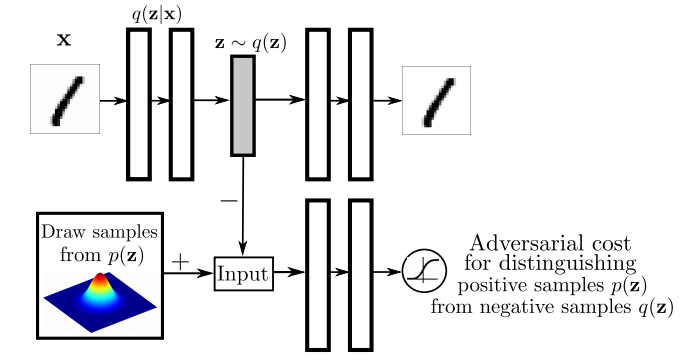
The top part of this image is a probabilistic autoencoder. Given the input $\mathbf{x}$, some latent code $\mathbf{z}$ is generated by sampling from an encoding distribution $q(\mathbf{z}\vert\mathbf{x})$. This distribution is typically modeled as the output a deep neural network. In normal autoencoders this encoder would be deterministic, now we allow it to be probabilistic.
A decoder network is then trained to decode $\mathbf{z}$ and reconstruct the original input $\mathbf{x}$. Of course, reconstruction will not be perfect, but we train the networks to minimise reconstruction error, this is typically just mean squared error.
The reconstruction cost ensures that the encoding process retains information about the input image, but it doesn't enforce anything else about what these latent representations $\mathbf{z}$ should do. In general, their distribution is described as the aggregate posterior $q(\mathbf{z})=\mathbb{E}_\mathbf{x} q(\mathbf{z}\vert\mathbf{x})$. Often, we would like this distribution to match a certain prior $p(\mathbf{z})$. For example. we may want $\mathbf{z}$ to have independent components and Gaussian distributed (nonlinear ICA,PCA). Or we may want to force the latent representations to correspond to discrete class labels, or binary factors. Or we may simply want to ensure there are 'no gaps' in the latent space, and any random $\mathbf{z}$ would lead to a viable sample when squashed through the decoder network.
So there are multiple reasons why one might want to control the aggregate posterior $q(\mathbf{z})$ to match a predefined prior $p(\mathbf{z})$. The authors achieve this by introducing an additional term in the autoencoder loss function, one that measures the divergence between $q$ and $p$. The authors chose to do this via adversarial training: they train a discriminator network that constantly learns to discriminate between real code vectors $\mathbb{z}$ produced by encoding real data, and random code vectors sampled from $p$. If $q$ matches $p$ perfectly, the optimal discriminator network should have a large classification error.
#### Is this an overkill?
My main question about this paper was whether the adversarial cost is really needed here, because I think it's an overkill. Let me explain:
Adversarial training is powerful when all else fails to quantify divergence between complicated, potentially degenerate distributions in high dimensions, such as images or video. Our toolkit for dealing with images is limited, CNNs are the best tool we have, so it makes sense to incorporate them in training generative models for images. GANs - when applied directly to images - are a great idea.
However, here adversarial training is applied to an easier problem: to quantify the divergence between a simple, fixed prior (e.g. Gaussian) and an empirical distribution of latents. The latent space is usually lower-dimensional, distributions better behaved. Therefore, matching to $p(\mathbf{z})$ in latent space should be considerably easier than matching distributions over images.
Adversarial training makes no assumptions about the distributions compared, other than sampling from them. This comes very handy when both $p$ and $q$ are nasty such as in the generative adversarial network scenario: there, $p$ is the distribution of natural images, $q$ is a super complicated, degenerate distribution produced by squashing noise through a deep convnet. The price we pay for this flexibility is this: when $p$ or $q$ are actually easy to work with, adversarial training cannot exploit that, it still has to sample. (it would be interesting to see if expectations over $p(\mathbf{z})$ could be computed analytically). So even though in this work $p$ is as simple as a mixture of ten 2D Gaussians, we need to approximate everything by drawing samples.
#### Other things might work: kernel moment matching
Why can’t one use easier divergences? For example, I think moment matching based on kernel MMD would work brilliantly in this scenario. It would have the following advantages over the adversarial cost.
- closed form expressions: Depending on the choice of the prior $p(\mathbf{z})$ and kernel used in MMD, the expectations over $p$ may be available in closed form, without sampling. So for example if we use a squared exponential kernel and a mixture of Gaussians as $p$, the divergence from $p$ can be precomputed in closed form that is easy to evaluate.
- no nasty inner loop: Adversarial training requires the discriminator network to be reoptimised every time the generative model changes. So we end up with a gradient descent in the inner loop of a gradient descent, which is anything but nice to work with. This is why it takes so long to get it working, the whole thing is pretty unstable. In contrast, to evaluate MMD, the inner loop is not needed. In fact, MMD can also be thought of as the solution to a convex maximisation problem, but via the kernel trick the maximum has a closed form solution.
- the problem is well suited for MMD: because the distributions are smooth, and the space is nice and low-dimensional, MMD might work very well. Kernel-based methods struggle with complicated manifold-like structure of natural images, so I wouldn't expect MMD to be competitive with adversarial training if it is applied directly in the image space. Therefore, I actually prefer generative adversarial networks to generative moment matching networks. However, here we have an easier problem, simpler space, simpler distributions where MMD shines, and adversarial training is just not needed.


