* They present a model which adds color to grayscale images (e.g. to old black and white images).
  * It works best with 224x224 images, but can handle other sizes too.

### How
  * Their model has three feature extraction components:
    * Low level features:
      * Receives 1xHxW images and outputs 512xH/8xW/8 matrices.
      * Uses 6 convolutional layers (3x3, strided, ReLU) for that.
    * Global features:
      * Receives the low level features and converts them to 256 dimensional vectors.
      * Uses 4 convolutional layers (3x3, strided, ReLU) and 3 fully connected layers (1024 -> 512 -> 256; ReLU) for that.
    * Mid-level features:
      * Receives the low level features and converts them to 256xH/8xW/8 matrices.
      * Uses 2 convolutional layers (3x3, ReLU) for that.
  * The global and mid-level features are then merged with a Fusion Layer.
    * The Fusion Layer is basically an extended convolutional layer.
    * It takes the mid-level features (256xH/8xW/8) and the global features (256) as input and outputs a matrix of shape 256xH/8xW/8.
    * It mostly operates like a normal convolutional layer on the mid-level features. However, its weight matrix is extended to also include weights for the global features (which will be added at every pixel).
    * So they use something like `fusion at pixel u,v = sigmoid(bias + weights * [global features, mid-level features at pixel u,v])` - and that with 256 different weight matrices and biases for 256 filters.
  * After the Fusion Layer they use another network to create the coloring:
    * This network receives 256xH/8xW/8 matrices (merge of global and mid-level features) and generates 2xHxW outputs (color in L\*a\*b\* color space).
    * It uses a few convolutional layers combined with layers that do nearest neighbour upsampling.
  * The loss for the colorization network is a MSE based on the true coloring.
  * They train the global feature extraction also on the true class labels of the used images.
  * Their model can handle any sized image. If the image doesn't have a size of 224x224, it must be resized to 224x224 for the gobal feature extraction. The mid-level feature extraction only uses convolutions, therefore it can work with any image size. 

### Results
  * The training set that they use is the "Places scene dataset".
  * After cleanup the dataset contains 2.3M training images (205 different classes) and 19k validation images.
  * Users rate images colored by their method in 92.6% of all cases as real-looking (ground truth: 97.2%).
  * If they exclude global features from their method, they only achieve 70% real-looking images.
  * They can also extract the global features from image A and then use them on image B. That transfers the style from A to B. But it only works well on semantically similar images.

![Architecture](https://raw.githubusercontent.com/aleju/papers/master/neural-nets/images/Let_there_be_Color__architecture.png?raw=true "Architecture")

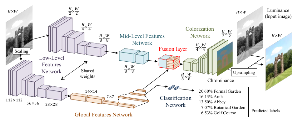
*Architecture of their model.*


![Old images](https://raw.githubusercontent.com/aleju/papers/master/neural-nets/images/Let_there_be_Color__old_images.png?raw=true "Old images")

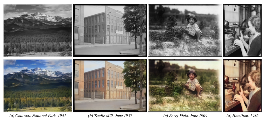
*Their model applied to old images.*

--------------------

# Rough chapter-wise notes

* (1) Introduction
  * They use a CNN to color images.
  * Their network extracts global priors and local features from grayscale images.
  * Global priors:
    * Extracted from the whole image (e.g. time of day, indoor or outdoors, ...).
    * They use class labels of images to train those. (Not needed during test.)
  * Local features: Extracted from small patches (e.g. texture).
  * They don't generate a full RGB image, instead they generate the chrominance map using the CIE L\*a\*b\* colorspace.
  * Components of the model:
    * Low level features network: Generated first.
    * Mid level features network: Generated based on the low level features.
    * Global features network: Generated based on the low level features.
    * Colorization network: Receives mid level and global features, which were merged in a fusion layer.
  * Their network can process images of arbitrary size.
  * Global features can be generated based on another image to change the style of colorization, e.g. to change the seasonal colors from spring to summer.

* (3) Joint Global and Local Model
  * <repetition of parts of the introduction>
  * They mostly use ReLUs.
  * (3.1) Deep Networks
    * <standard neural net introduction>
  * (3.2) Fusing Global and Local Features for Colorization
    * Global features are used as priors for local features.
    * (3.2.1) Shared Low-Level Features
      * The low level features are which's (low level) features are fed into the networks of both the global and the medium level features extractors.
      * They generate them from the input image using a ConvNet with 6 layers (3x3, 1x1 padding, strided/no pooling, ends in 512xH/8xW/8).
    * (3.2.2) Global Image Features
      * They process the low level features via another network into global features.
      * That network has 4 conv-layers (3x3, 2 strided layers, all 512 filters), followed by 3 fully connected layers (1024, 512, 256).
      * Input size (of low level features) is expected to be 224x224.
    * (3.2.3) Mid-Level Features
      * Takes the low level features (512xH/8xW/8) and uses 2 conv layers (3x3) to transform them to 256xH/8xW/8.
    * (3.2.4) Fusing Global and Local Features
      * The Fusion Layer is basically an extended convolutional layer.
      * It takes the mid-level features (256xH/8xW/8) and the global features (256) as input and outputs a matrix of shape 256xH/8xW/8.
      * It mostly operates like a normal convolutional layer on the mid-level features. However, its weight matrix is extended to also include weights for the global features (which will be added at every pixel).
      * So they use something like `fusion at pixel u,v = sigmoid(bias + weights * [global features, mid-level features at pixel u,v])` - and that with 256 different weight matrices and biases for 256 filters.
    * (3.2.5) Colorization Network
      * The colorization network receives the 256xH/8xW/8 matrix from the fusion layer and transforms it to the 2xHxW chrominance map.
      * It basically uses two upsampling blocks, each starting with a nearest neighbour upsampling layer, followed by 2 3x3 convs.
      * The last layer uses a sigmoid activation.
      * The network ends in a MSE.
  * (3.3) Colorization with Classification
    * To make training more effective, they train parts of the global features network via image class labels.
    * I.e. they take the output of the 2nd fully connected layer (at the end of the global network), add one small hidden layer after it, followed by a sigmoid output layer (size equals number of class labels).
    * They train that with cross entropy. So their global loss becomes something like `L = MSE(color accuracy) + alpha*CrossEntropy(class labels accuracy)`.
  * (3.4) Optimization and Learning
    * Low level feature extraction uses only convs, so they can be extracted from any image size.
    * Global feature extraction uses fc layers, so they can only be extracted from 224x224 images.
    * If an image has a size unequal to 224x224, it must be (1) resized to 224x224, fed through low level feature extraction, then fed through the global feature extraction and (2) separately (without resize) fed through the low level feature extraction and then fed through the mid-level feature extraction.
    * However, they only trained on 224x224 images (for efficiency).
    * Augmentation: 224x224 crops from 256x256 images; random horizontal flips.
    * They use Adadelta, because they don't want to set learning rates. (Why not adagrad/adam/...?)

* (4) Experimental Results and Discussion
  * They set the alpha in their loss to `1/300`.
  * They use the "Places scene dataset". They filter images with low color variance (including grayscale images). They end up with 2.3M training images and 19k validation images. They have 205 classes.
  * Batch size: 128.
  * They train for about 11 epochs.
  * (4.1) Colorization results
    * Good looking colorization results on the Places scene dataset.
  * (4.2) Comparison with State of the Art
    * Their method succeeds where other methods fail.
    * Their method can handle very different kinds of images.
  * (4.3) User study
    * When rated by users, 92.6% think that their coloring is real (ground truth: 97.2%).
    * Note: Users were told to only look briefly at the images.
  * (4.4) Importance of Global Features
    * Their model *without* global features only achieves 70% user rating.
    * There are too many ambiguities on the local level.
  * (4.5) Style Transfer through Global Features
    * They can perform style transfer by extracting the global features of image B and using them for image A.
  * (4.6) Colorizing the past
    * Their model performs well on old images despite the artifacts commonly found on those.
  * (4.7) Classification Results
    * Their method achieves nearly as high classification accuracy as VGG (see classification loss for global features).
  * (4.8) Comparison of Color Spaces
    * L\*a\*b\* color space performs slightly better than RGB and YUV, so they picked that color space.
  * (4.9) Computation Time
    * One image is usually processed within seconds.
    * CPU takes roughly 5x longer.
  * (4.10) Limitations and Discussion
    * Their approach is data driven, i.e. can only deal well with types of images that appeared in the dataset.
    * Style transfer works only really well for semantically similar images.
    * Style transfer cannot necessarily transfer specific colors, because the whole model only sees the grayscale version of the image.
    * Their model tends to strongly prefer the most common color for objects (e.g. grass always green).

TLDR; The authors propose two LSTM-based models for target-dependent sentiment classification. TD-LSTM uses two LSTM networks running towards to target word from left and right respectively, making a prediction at the target time step. TC-LSTM is the same, but additionally incorporates the an averaged target word vector as an input at each time step. The authors evaluate their models with pre-trained word embeddings on a Twitter sentiment classification dataset, achieving state of the art.

#### Key Points

- TD-LSTM: Two LSTM networks, running from left to right towards the target. The final states of both networks are concatenated and the prediction is made at the target word.
- TC-LSTM: Same architecture as TD-LSTM, but also incorporates the word vector as an input at each time step. The word vector is the average of the word vectors for the target phrase.
- Embeddings seem to make a huge difference, state of the art is only obtained with 200-dimensional GloVe embeddings.


#### Notes/Questions

- A *huge* fraction of the performance improvement comes from pre-trained word embeddings. Without these, the proposed models clearly underperforms simpler models. This raises the question of whether incorporating the same embeddings into the simpler models would do.
- Would've liked to see performance without *any* pre-trained embeddings.
- The authors also experimented with attention mechanisms, but weren't able to achieve good results. Small size of training corpus may be the reason for this.

This week I read upon [GraphX](https://amplab.cs.berkeley.edu/wp-content/uploads/2014/02/graphx.pdf), a distributed graph computation framework that unifies graph-parallel and data-parallel computation. Graph-parallel systems efficiently express iterative algorithms (by exploiting the static graph structure) but do not perform well on operations that require a more general view of the graph like operations that move data out of the graph. Data-parallel systems perform well on such tasks but directly implementing graph algorithms on data-parallel systems is inefficient due to complex joins and excessive data movement. This is the gap that GraphX fills in by allowing the same data to be viewed and operated upon both as a graph and as a table.

### Preliminaries

Let $G = (V, E)$ be a graph where $V = \{1, ..., n\}$ is the set of vertices and $E$ is the set of $m$ directed edges. Each directed edge is a tuple of the form $(i, j)  \in E$ where $i \in V$ is the source vertex and $j \in V$ is the target vertex. The vertex properties are represented as $P_V(i)$ where $i \in V$ and edge properties as $P_E (i, j)$ for edge $(i, j) \in E$. The collection of all the properties is $P = (P_V, P_E)$. The combination of graph structure and properties defines a property graph $G(P) = (V, E, P)$.

Graph-Parallel Systems consist of a property graph $G = (V, E, P)$ and a vertex-program $Q$ that is instantiated simultaneously on all the vertices. The execution on vertex $v$, called $Q(v)$, interacts with execution on the adjacent vertices by message passing or shared state and can read/modify properties on the vertex, edges and adjacent vertices. $Q$ can run in two different modes:

* **bulk-synchronous mode** - all vertex programs run concurrently in a sequence of super-steps. 
* **asynchronous mode** - vertex programs run as and when resources are available and impose constraints on whether neighbouring vertex-programs can run concurrently.

**Gather-Apply-Scatter (GAS)** decomposition model breaks down a vertex-program into purely edge-parallel and vertex-parallel stages. The associative *gather* function collects the inbound messages on the vertices, the *apply* function operates only on the vertices and updates its value and the *scatter* function computes the message to be sent along each edge and can be safely executed in parallel.

GrapX uses bulk-synchronous model and adopts the GAS decomposition model.

### GraphX Data Model

The GraphX Data Model consists of immutable collections and property graphs. Collections consist of unordered tuples (key-value pairs) and are used to represent unstructured data. The property graph combines the structural information (in the form of collections of vertices and edges) with properties describing this structure. Properties are just collections of form $(i, P_V (i))$ and $((i, j), P_E (i, j))$. The collection of vertices and edges are represented using RDDs (Resilient Distributed Datasets). Edges can be partitioned as per a user defined function. Within a partition, edges are clustered by source vertex id and there is an unclustered index on target vertex id. The vertices are hash partitioned by id and stored in a hash index within a partition. Each vertex partition contains a bitmask which allows for set intersection and filtering. It also contains a routing table that logically maps a vertex id to set of edge partitions containing the adjacent edges. This table is used when constructing triplets and is stored as a compressed bitmap.

### Operators

Other than standard data-parallel operators like `filter`, `map`, `leftJoin`, and `reduceByKey`, GraphX supports following graph-parallel operators:
*   `graph` - constructs property graph given a collection of edges and vertices.
*   `vertices`, `edges` - decompose the graph into a collection of vertices or edges by extracting vertex or edge RDDs.
*   `mapV`, `mapE` - transform the vertex or edge collection.
*   `triplets` -returns collection of form $((i, j), (P_V (i), P_E (i, j), P_V (j)))$. The operator essentially requires a multiway join between vertex and edge RDD. This operation is optimized by shifting the site of joins to edges, using the routing table, so that only vertex data needs to be shuffled.    
*   `leftJoin` - given a collection of vertices and a graph, returns a new graph which incorporates the property of matching vertices from the given collection into the given graph without changing the underlying graph structure.
*   `subgraph` - returns a subgraph of the original graph by applying predicates on edges and vertices
*   `mrTriplets` (MapReduce triplet) - logical composition of triplets followed by map and reduceByKey. It is the building block of graph-parallel algorithms.

All these operators can be expressed in terms on relational operators and can be composed together to express different graph-parallel abstractions. The paper shows how these operators can be used to construct a enhanced version of Pregel based on GAS. It also shows how to express connected components algorithm and `coarsen` operator.

### Structural Index Reuse

Collections and graphs, being immutable, share the structural indexes associated within each vertex and edge partition to both reduce memory overhead and accelerate local graph operations. Most of the operators preserve the structural indexes to reuse them. For operators like subgraph which restrict the graph, the bitmask is used to construct the restricted view. 

### Distributed Join Optimization

##### Incremental View Maintenance

The number of vertices that change between different steps of iterative graph algorithms decreases as the computation converges. After each operation, GraphX tracks which vertices have been changed by maintaining a bit mask. When materializing a vertex view, it uses values from the previous view for vertices which have not changed and ships only those vertices which are changed. This also allows for another optimization when using the `mrTriplets` operation: `mrTriplets` support an optional argument called *skipStale*. when this option is enabled, the `mrTriplets` function does not apply on edges origination from vertices that have not changed since its last iteration. This optimization uses the same bitmask that incremental views were using.  

##### Automatic Join elimination

GraphX has implemented a JVM bytecode analyzer that determines whether source/target vertex attributes are referenced in a mrTriplet UDF (for map) or not. Since edges already contain the vertex ids, a 3-way join can be brought down to 2-way join if only source/target vertex attributes are needed (as in PageRank algorithm) or the join can be completely eliminated if none of the vertex attributes are referenced.

### Sequential Scan vs Index Scan

Using structural indices, while reduces computation cost in iterative algorithms, prevents physical data from shrinking. To counter this issue, GraphX switches from sequential scan to bitmap index scan when the fraction of active vertices drops below 0.8. Since edges are clustered by source vertex id, bitmap index scan can efficiently join edges and vertexes together.

### Other Optimizations

* Though GraphX uses Spark's shuffle mechanism, it materializes shuffled data in memory itself, unlike Spark which materializes shuffle data in disk and relies on OS buffer cache to cache the data. The rationale behind this modification is that graph algorithms tend to be communication intensive and inability to control when buffers are flushed can lead to additional overhead.
* When implementing join step, vertices routed to the same target are batched, converted from row-orientation to column-orientation and compressed by LZF algorithm and then sent to their destination.
* During shuffling, integers are encoded using a variable encoding scheme where for each byte, the first 7 bits encode the value, and the highest order bit indicates if another byte is needed for encoding the value. So smaller integers can be encoded with fewer bytes and since, in most cases, vertex ids are smaller than 64 bits, the technique helps to reduce an amount of data to be moved.


### System Evaluation

GraphX was evaluated against graph algorithms implemented over Spark 0.8.1, Giraph 1.0 and GraphLab 2.2 for both graph-parallel computation tasks and end-to-end graph analytic pipelines. Key observations:


*    GraphLab benefits from its native runtime and performs best among all the implementations for both PageRank and Connected Components algorithm.
*    For connected components algorithm, Giraph benefits from using edge cuts but suffers from Hadoop overhead.
*    GraphX outperforms idiomatic implementation of PageRank on Spark, benefitting from various optimizations discussed earlier. 
*    As more machines are added, GraphX does not scale linearly but it still outperforms the speedup achieved by GraphLab (for PageRank).
*    GraphX outperforms Giraph and GraphLab for a multi-step, end-to-end graph analytics pipeline that parses Wikipedia articles to make a link graph, runs PageRank on the link graph and joins top 20 articles with their text.


GraphX provides a small set of core graph-processing operators, implemented on top of relational operators, by efficiently encoding graphs as a collection of edges and vertices with two indexing data structures. While it does lag behind specialised systems like Giraph and GraphLab in terms of graph-parallel computation tasks, GraphX does not aim at speeding up such tasks. It instead aims to provide an efficient workflow in end-to-end graph analytics system by combining data-parallel and graph-parallel computations in the same framework. Given that it does outperform all the specialised systems in terms of end-to-end runtime for graph pipelines and makes the development process easier by eliminating the need to learn and maintain multiple systems, it does seem to be a promising candidate for the use case it is attempting to solve.

## Keywords
Triplet-loss , face embedding , harmonic embedding

---
## Summary

### Introduction

**Goal of the paper**    
A unified system is given for face verification , recognition and clustering.
Use of a 128 float  pose and illumination invariant feature vector or embedding in the euclidean space.
* Face Verification : Same faces of the person gives feature vectors that have a very close L2 distance between them. 
* Face recognition : Face recognition becomes a clustering task in the embedding space
	
**Previous work**    
* Previous use of deep learning made use of an bottleneck layer to represent face as an embedding of  1000s  dimension  vector.
* Some other techniques use PCA to reduce the dimensionality of the embedding for comparison.

**Method**
* This method makes use of inception style CNN to get an embedding of each face.
* The thumbnails of the face image are the tight crop of the face area with only scaling and translation done on them.
	
**Triplet Loss**
Triplet loss  makes use of two matching face thumbnails and a non-matching thumbnail. The loss function tries to reduce the distance between the matching pair while increasing the separation between the the non-matching pair of images.

**Triplet Selection**
* Selection of triplets is done such that samples are hard-positive or hard-negative .
* Hardest negative can lead to local minima early in the training and a collapse model in a few cases
* Use of semi-hard negatives help to improve the convergence speed while at the same time reach nearer to the global minimum.

**Deep Convolutional Network**
* Training is done using SGD (Stochastic gradient descent) with Backpropagation and AdaGrad
* The training is done on two networks :
    - Zeiler&Fergus architecture with model depth of 22 and 140 million parameters
    - GoogLeNet style inception model with 6.6 to 7.5 million parameters.

**Experiment**
* Study of the following cases are done :
    - Quality of the jpeg image : The validation rate of model improves with the JPEG quality upto a certain threshold.

    - Embedding dimensionality : The dimension of the embedding increases from 64 to 128,256 and then gradually starts to decrease at 512 dimensions. 

    - No. of images in the training data set 



**Results classification accuracy** :
   - LFW(Labelled faces in the wild) dataset : 98.87% 0.15
   - Youtube Faces DB : 95.12%  .39
On clustering tasks the model was able to work on a wide varieties of face images and is invariant to pose , lighting and also age.

**Conclusion**

* The model can be extended further to improve the overall accuracy.
* Training networks to run on smaller systems like mobile phones.
* There is need for improving the training efficiency.

---

## Notes 

* Harmonic embedding is a set of embedding that we get from different models but are compatible to each other. This helps to improve future upgrades and transitions to a newer model

* To make the embeddings compatible with different models , harmonic-triplet loss and the generated triplets must be compatible with each other

## Open research questions

* Better understanding of the error cases.
* Making the model more compact for embedded and mobile use cases.
* Methods to reduce the training times.

This paper introduces an interpretation of deep residual networks as implicit ensembles of exponentially many shallow networks. For a residual block $i$, there are $2^{i-1}$ paths from input to $i$, and the input to $i$ is a mixture of  $2^{i-1}$ different distributions. The interpretation is backed by a number of experiments such as removing or re-ordering residual blocks at test time and plotting norm of gradient v/s number of residual blocks the gradient signal passes through. Removing $k$ residual blocks (for k <= 20) from a network of depth n decreases the number of paths to $2^{n-k}$ but there are still sufficiently many valid paths to not hurt classification error, whereas sequential CNNs have a single viable path which gets corrupted. Plot of gradient at input v/s path length shows that almost all contributions to the gradient come from paths shorter than 20 residual blocks, which are the effective paths. The paper concludes by saying that network 'multiplicity', which is the number of paths, plays a key role in terms of the network's expressability.

## Strengths

- Extremely insightful set of experiments. These experiments nail down the intuitions as to why residual networks work, as well as clarify the connections with stochastic depth (sampling the network multiplicity during training i.e. ensemble by training) and highway networks (reduction in number of available paths by gating both skip connections and paths through residual blocks).

## Weaknesses / Notes

- Connections between effective paths and model compression.