#### Explainability-Accuracy trade-off

Many practical applications of machine learning systems call for the ability to explain why certain predictions are made. Consider a fraud detection system: it is not very useful for a user to see a list of possible fraud attempts without any explanation why the system thought the attempt was fraud. You want to say something like 'the system thinks it's fraud because the credit card was used to make several transactions that are smaller than usual'. But such explanations are not always compatible with our machine learning model. Or are they?

When choosing a machine learning model we usually think in terms of two choices:

- accurate but black-box: The best classification accuracy is typically achieved by black-box models such as Gaussian processes, neural networks or random forests, or complicated ensembles of all of these. Just look at the kaggle leaderboards. These are called black-box and are often criticised because their inner workings are really hard to understand. They don't, in general, provide a clear explanation of the reasons they made a certain prediction, they just spit out a probability.

- white-box but weak: On the other end of the spectrum, models whose predictions are easy to understand and communicate are usually very impoverished in their predictive capacity (linear regression, a single decision tree) or are inflexible and computationally cumbersome (explicit graphical models).

So which ones should we use: accurate black-box models, or less accurate but easy-to-explain white-box models?

The paper basically tells us that this is a false tradeoff. To summarise my take-home from this poster in one sentence:

`Explainability is not a property of the model`

Ryan presents a nice way to separate concerns of predictive power and explanation generation. He does this by introducing a formal framework in which simple, human-readable explanations can be generated for any black-box classifier, without assuming anything about the internal workings of the classifier.

If you think about it, it makes sense. If you watch someone playing chess, you can probably post-rationalise and give a reason why the person might think it's a good move. But you probably don't have an idea about the algorithm the person was executing in his brain.

Now we have a way to explain why decisions were made by complex systems, even if that explanation is not an exact explanation of what the classifier algorithm actually did. This is super-important in applications such as face recognitions where the only models that seem to work today are large black-box models. As (buzzword alert) AI-assisted decision making is becoming commonplace, the ability to generate simple explanations for black-box systems is going to be super important, and I think Ryan has made some very good observations in this paper.

I recommend everyone to take a look, I'm definitely going to see the world a bit differently after reading this.

### Evaluating Generative Models

A key topic I'm very interested in is the choices of objective functions used in unsupervised learning and generative models. The key organising principle should be this: the objective function we use for training a probabilistic model should match the way we ultimately want to use the model. Yet, in unsupervised learning this is often overlooked and I think we lack clarity around what the models are used for and how they should be trained and evaluated. This paper tries to clarify this a bit in the context of generative models. I also want to mention that another ICLR submission this year also deals with this fundamental question: I highly recommend taking a look.

Here, I'm going to consider a narrow definition of generative models: models we actually want to use to generate samples from which are then shown to a human user/observer. This includes use-cases such as image captioning, texture generation, machine translation, speech synthesis and dialogue systems, but excludes things like unsupervised pre-training for supervised learning, semisupervised learning, data compression, denoising and many others. Very often people don't make this distinction clear when talking about generative models which is one of the reasons why there is still no clarity about what different objective functions do.

I argue that when the goal is to train a model that can generate natural-looking samples, maximum likelihood is not a desirable training objective. Maximum likelihood is consistent so it can learn any distribution if it is given infinite data and a perfect model class. However, under model misspecification and finite data (that is, in pretty much every practically interesting scenario), it has a tendency to produce models that overgeneralise.

#### KL divergence as a perceptual loss

Generative modelling is about finding a probabilistic model $Q$ that in some sense approximates the natural distribution of data $P$. When researchers (or users of their product) evaluate generative models for perceptual quality, they draw samples from it, then - for lack of a better word - eyeball the samples. In visual information processing this is often referred to as no-reference perceptual quality assessment \citep[see e.,g.\ ][]{wang2002noreference}. In the paper, I propose that the KL divergence $KL[Q\| P]$ can be used as an idealised objective function to describe this scenario. This related to maximum likelihood which minimises $KL[P\|Q]$, but different in fundamental ways which I will explain later.

Here is why I think $KL[Q\|P]$ should be used: First, we can make the assumption that the perceived quality of each sample is related to the \emph{surprisal} $-\log Q_{human}(x)$ under the human observers' subjective prior of stimuli $Q_{human}(x)$. For those of you not familiar with computational cognitive science, this will seem ad-hoc, but it's a relatively common assumption to make when modelling reaction times in experiments for example. We further assume that the human observer maintains a very accurate model of natural stimuli, thus, $Q_{human}(x) \approx P(x)$. This is a fancy way of saying things like the observer being a native speaker therefore understanding all the nuances in language. These two assumptions suggest that in order to optimise our chances in this Turing test-like scenario, we need to minimise the following cross-entropy or perplexity term:

\begin{equation} - \mathbb{E}_{x\sim Q} \log P(x) \end{equation}

This perplexity is the exact opposite average negative log likelihood $- \mathbb{E}_{x\sim P} \log Q(x)$, with the role of $P$ and $Q$ changed. However, the perplexity alone would be maximised by a model $Q$ that deterministically picks the most likely stimulus. To enforce diversity one can simultaneously try to maximise the Shannon entropy of $Q$. This leaves us with the following KL divergence to optimise:

\begin{equation} KL[Q\| P] = - \mathbb{E}{x\sim Q} \log P(x) + \mathbb{E}{x\sim Q} \log Q(x) \end{equation}

So if we want to train models that produce nice samples, my recommendation is to try to use $KL[Q\|P]$ as an objective function or something that behaves like it. How does maximum likelihood compare?

#### Differences between maximum likelihood and $KL[Q\|P]$

Maximum likelihood is roughly the same as minimising $KL[P\|Q]$. The differences between minimising $KL[P\|Q]$ and $K[Q\|P]$ are well understood and it frequently comes up in the context of Bayesian approximate inference as well. Both divergences ensure consistency, minimising either converges to the true $P$ in the limit of infinite data and a perfect model class. However, they differ fundamentally in the way they deal with finite data and model misspecification (in almost every practical scenario):

$KL[P\|Q]$ tends to favour approximations $Q$ that overgeneralise $P$. If P is multimodal, the optimal $Q$ will tend to cover all the modes of $P$, even at the cost of introducing probability mass where $P$ has $0$ mass. Practically this means that the model will occasionally sample unplausible samples that don't look anything like samples from $P$.
$KL[Q\|P]$ tends to favour under-generalisation. The optimal $Q$ will typically describe the single largest mode of $P$ well, at the cost of ignoring other modes if they are hard to model without covering low-probability areas as well. Practically this means that $KL[Q\|P]$ will try to avoid introducing unplausible samples, sometimes at the cost of missing the majority of plausible samples under $P$.
In other words: $KL[P\|Q]$ is liberal, $KL[Q\|P]$ is conservative. In yet other words: $KL[P\|Q]$ is an optimist, $KL[Q\|P]$ is a pessimist.

The problem of course is that $KL[Q\|P]$ is super hard to optimise beased on a finite sample from $P$. Even harder than maximum likelihood. Not only that, the KL divergence is also not very well behaved, and is not well-defined unless $P$ is positive everywhere where $Q$ is positive. So there is little hope we can turn $KL[Q\|P]$ into a practical training algorithm.

#### Generalised Adversarial Training

Generative Adversarial Networks(GANs) train a generative model jointly with an adversarial discriminative model that tries to differentiate between artificial and real data. The idea is, a generative model is good if it can fool the best discriminative model into thinking the generated samples are real. GANs have produced some of the nicest looking samples you'll find on the Internet and got people very excited about generative models again: human faces, album covers, etc.

How do they come into this picture? It's because they can be understood as approximately minimising the Jensen-Shannon divergence:

\begin{equation} JSD[P\|Q] = JSD[P\|Q] = \frac{1}{2}KL\left[P\middle\|\frac{P+Q}{2}\right] + \frac{1}{2}KL\left[Q\middle\|\frac{P+Q}{2}\right]. 
\end{equation}

Looking at the equation above you can immediately see how it's related to this topic. JS divergence is a bit like a symmetrised version of KL divergence. It's not $KL[P\|Q]$, not $KL[Q\|P]$, but a bit of both. So one can expect that minimising JS divergence would exhibit a behaviour that is kind of halfway between the two extremes explained above. And that means that they would generate better samples than methods trained via maximum likelihood and similar objectives.

What's more, one can generalise JS divergence to a whole family of divergences, parametrised by a probability $0<\pi<1$ as follows:

\begin{equation} JS_{\pi}[P\|Q] = \pi \cdot KL[P\|\pi P+(1-\pi)Q] + (1-\pi)KL[Q\|\pi P+(1-\pi)Q]. 
\end{equation}

What I show in the paper is that by varrying $\pi$ between the two extremes, one can effectively interpolate between the behaviour of maximum likelihood ($\pi\rightarrow 0$) and minimising $KL[Q\|P]$ ($\pi\rightarrow 1$). See the paper for details. This interpolation between behaviours is explained in this main figure below:

![](http://www.inference.vc/content/images/2015/11/Screen-Shot-2015-11-16-at-16-19-10.png)

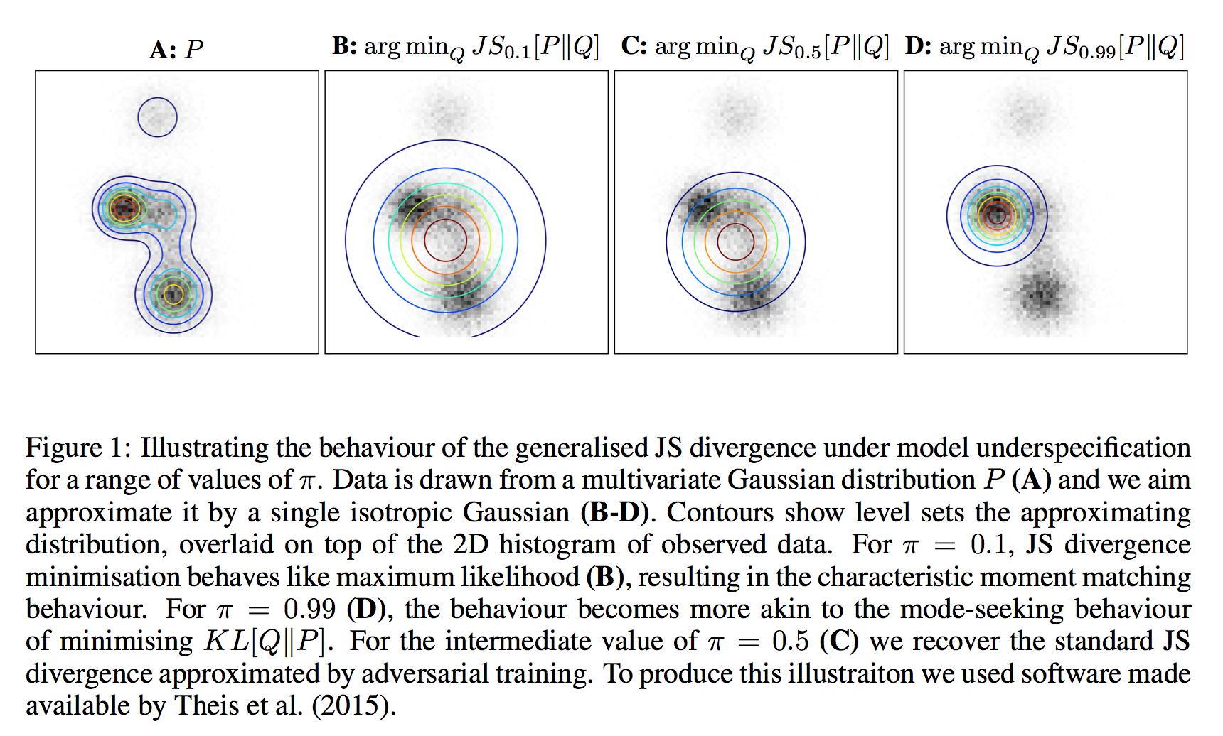
For any given value of $\pi$, we can optimise $JS_{\pi}$ approximately using an algorithm that is a slightly changed version of the original GAN algorithm. This is because the generalised JS divergence still has an elegant information theoretic interpretation. Consider a communications channel on which we can transmit a single data point of some kind. We toss a coin and with probability $\pi$, we send a sample from $P$, and with probability $1-\pi$ we send a sample from $Q$ instead. The receiver doesn't know the outcome of the coinflip, she only observes the sample. The $JS_{\pi}$ is the mutual information between the observed sample and the coinflip. It is also an upper bound on how well any algorithm can do in guessing the coinflip from the observed sample.

To implement an adversarial training algorithm for $JS_{\pi}$ one simply needs to change the ratio of samples the discriminative network sees from $Q$ vs $P$ (or apply appropriate weights during training). In the original method the discriminator network is faced with a balanced classification problem, i.e. $\pi=\frac{1}{2}$. It is hard to believe, but this irrelevant-looking modification changes the behaviour of the GAN algorithm dramatically, and can in theory allow the GAN algorithm to approximate both maximum likelihood or $KL[Q\|P]$.

This analysis explains why GANs have been so successful in generating very nice looking images, and relatively few weird-looking ones. It is also worth pointing out that the GAN method is still in its infantcy and has many issues and limitations. The main issue is that it is based on sampling from $Q$ which doesn't work well in high dimensions. Hopefully some of these limitations can be overcome and then we should have a pretty powerful framework for training good generative models.

Google's team developed scheduled sampling as an alternative training procedure to fit RNNs, and they used it in their competition-winning method for image captioning. While I can't argue with the empirical results (so I won't), I was a bit skeptical about the technique at a fundamental level, so I decided to do a bit of math that resulted in this blog post.

Overall, I have a suspicion that scheduled sampling is a flawed objective function for unsupervised/generative modelling, and I want to use this post to explain why I think so. I hope the comments section will work this time so people can comment and argue otherwise. Please also shoot me an email if you have more to say.

#### Summary of this note

- I have a critical look at scheduled sampling as objective function for training RNNs
- I show it can lead to pathologies where the RNN learns marginal instead of conditional distributions
- I explain why I think adversarial training/generative moment matching offers a better alternative
- Lastly, I include a paragraph in which I apologise for being a di*k again.

#### Strictly proper scoring rules

I've mentioned scoring rules on this blog many times, and my PhD thesis was about them, so saying I'm obsessed with this topic would be a valid observation. But this is important stuff, particularly for unsupervised learning, and particularly as a framework to think about hard concepts like overfitting in generative models.

Scoring rules are essentially loss functions for probabilistic models/forecasts. A scoring rule $$S(x,Q)$$ simply measures how bad a probabilistic forecast $Q$ for a variable is in the light of actual observation $x$. In this notation, lower is better. A scoring rule is called strictly proper, if for any $P$, the following holds:

$$\underset{Q}{\operatorname{argmax}} \mathbb{E}_{x\sim P}S(x,Q) = P$$

In other words, if you repeatedly sample observations from some true underlying distribution $P$, then the model $Q$ which minimises expected score is $P$. This means that the scoring rule cannot be fooled and that minimising the expected score yields a consistent estimator for $P$. Because I mention consistency, people may dismiss this as a learning theory argument, but it is not. If you are a Bayesian or a deep learning person with no interest in consistency, a scoring rule being strictly proper simply means that it is safe to use it as a loss function. Anything that's not strictly proper is weird and wrong, it will lead to learning the wrong thing.

This concept is central in unsupervised learning and generative modelling. Unsupervised learning is all about modelling the probability distribution of data, so it's essential that we have loss functions that can measure the discrepancy between our model $Q$, and the true data distribution $P$ in a consistent way.

#### log-likelihood

One of the most frequently used strictly proper scoring rule is the logarithmic score:

$$S(x,Q) = - \log Q(x)$$

This quantity is also known as the negative log-likelihood. Minimising the expected score in an i.i.d scenario yields maximum likelihood estimation, which is known to be a consistent estimator and has nice properties.

Often, the likelihood is impossible to evaluate. Luckily, it is not the only strictly proper scoring rule. In the context of generative models people have used the pseudolikelihood, score matching and moment matching, all of which are examples of strictly proper scoring rules.

To recap, any learning method that corresponds to minimising a strictly proper scoring rule is fine, everything else can go horribly wrong, even if we feed it infinite data, it might just learn the wrong thing.

#### Scheduled Sampling

After successfully establishing myself as a proper-scoring-rule-nazi, let's talk about scheduled sampling (SS). I don't have a lot of space explaining SS in great detail here, only the basic idea. I encourage everyone to read the paper and Hugo's summary above.

SS is a new method to train recurrent neural networks(RNNs) to model sequences. I will use character-by-character models of text as an example. Typically, when you train an RNN, you aim to minimise the log predictive likelihood in predicting the next character in each training sentence, given the prefix string of previous characters. This can be thought of as a special case of maximum likelihood learning, and is all fine, you can actually do this properly without approximations.

After training, you use the RNN to generate sample sentences in a recursive fashion: assuming you've already generated $n$ characters, you feed that prefix into the RNN, and ask it to predict the $n+1$st character. The $n+1$st character is then added to the prefix to predict the $n+2$th character, and so on.

The authors say there is a disconnect between how the model is trained (it's always fed real data) and how it's used (it's always fed synthetic data generated by itself). This, they argue, leads to the RNN being unable to recover from its own mistakes early on in the sentence.

To address this, the authors propose an alternative training strategy, where every once in a while, the network is given its own synthetic data instead of real data at training time. More specifically, for each character in the training sentences, we flip a coin to decide whether we feed the character from the real training sentence, or whether to feed the model's own prediction as to what that character would have been. The authors claim this makes the model more robust to recovering from mistakes, which is probably true.

As far as I'm concerned, I'm happy as long as the new training procedure corresponds to a strictly proper scoring rule. But in this case, I have a strong feeling that it does not.

#### case study: sequence of two variables

For sake of simplicity, let's consider using scheduled sampling to learn the joint distribution of a sequence of just two random variables. This is probably the simplest (shortest) time series I can think of. So SS in this case works as follows: For each datapoint train the network to predict the real $x_1$. Then we flip a coin to decide whether to keep $x_1$ from the datapoint, or to replace it with a sample from the model $Q_{x_1}$. Then we train $Q_{x_2\vert x_1}$ on the $(x_1,x_2)$ pair obtained this way.

The scoring rule for selective sampling looks something like this:

$$ S(Q_{x_1,x_2},(x_1,x_2)) = - (1 - \epsilon) [ \mathbb{E}_{z \sim Q_{x_1}} \log Q_{x_2 \vert x_1}(x_2 \vert z) + \log Q_{x_1}(x_1)] - \epsilon \log Q_{x_2 , x_1}(x_1,x_2),$$

where $\epsilon$ is the probability with wich the true $x_1$ is used.

The authors suggest starting training with $\epsilon=1$ and annealing it so that by the end of the training $\epsilon=0$. So as far as the eventual optimum of SS is concerned, we only have to focus on what the first term of the scoring rule does. The second term is the good old log-likelihood so we know that part works.

After some math, one can show that scheduled sampling with a fixed $\epsilon$ minimises the following divergence between the true $P$ and the model $Q$:

$$D_{SS}[P\|Q] = KL[P_{x_1}\|Q_{x_1}] + (1-\epsilon) \mathbb{E}_{z\sim Q_{x_1}} KL[P_{x_2}\|Q_{x_2\vert x_1=z}] + \epsilon KL[P_{x_2\vert x_1}\|Q_{x_2\vert x_1}]$$

Now, if $\epsilon=1$, we recover the Kullback-Leibler divergence between the joint $P_{x_1,x_2}$ and $Q_{x_1,x_2}$, which is what we expect as it corresponds to maximum likelihood estimation. However, as $\epsilon$ is annealed to $0$, the objective function is somewhat strange, whereby the conditional distribution $Q_{x_2\vert x_1}$ is pushed to model the marginal distribution $P_{x_2}$, instead of $P_{x_2\vert x_1}$ as one would expect. One can therefore see that the factorised $Q^{*} = P_{x_1}P_{x_2}$ minimises this objective function.

#### what this means for text modeling

Extrapolating from the two variable case to longer sequences, one can see that the scheduled sampling objective would fail if minimised properly until convergence. Consider the case when the $\epsilon\approx 0$ stage is reached in the annealing schedule. Now consider what the RNN has to do to predict the $n$th character in a string during training. It is fed a random prefix string that was generated by itself but never seen any real data. Then the RNN has to give a probabilistic forecast of what the $n$th character in the training sentence is, having seen none of the previous characters in the sentence.

The optimal model that minimises this objective would completely ignore all the characters in the sentence so far, but keep a simple linear counter that indexes where it is within the sentence. Then it would emit a character from an index-specific marginal distribution of characters. This is the equivalent of the factorised trivial solution above.

Yes, such a model would be better at "recovering from its own mistakes", because at every character it would start independently from what it has generated so far. But this is at the cost of paying no attention whatsoever as to what the prefix of the sentence was. I believe the reason why this trivial behaviour was not observed in the paper is that the authors did not run the optimisation until convergence, and did not implement the full gradient of the objective function, as they discuss in the paper.

#### Constructive part of criticism

#### What to do instead of SS?

So the observed problem was that RNNs trained via maximum likelihood are unable to recover from their own mistakes early on in a sentence, when they are used to generate.

`The main reason for the observed problem is that the log-likelihood is a local scoring rule`

The local property of scoring rules means that at training time we only ever evaluate the model $Q$ on actually observed datapoints. So if the RNN is faced with a prefix subsequence that was not in the dataset, God knows what it's going to complete that sentence with.

The proper (shall I say strictly proper) way to fix this issue is to use 

I think this paper has two main ideas in there, I see them as independent, for reasons explained below:

- A new penalty function that aims at regularising the second derivative of the trajectory the latent representation traces over time. I see this as a generalisation of the slowness principle or temporal constancy, more about this in the next section.

- A new autoencoder-like method to predict future frames in video. Video is really hard to forward-predict with non-probabilistic models because high level aspects of video are genuinely uncertain. For example, in a football game, you can't really predict whether the ball will hit the goalpost, but the results might look completely different visually. This, combined with L2 penalties often results in overly conservative, blurry predictions. The paper improves things by introducing extra hidden variables, that allow the model to represent uncertainty in its predictions. More on this later.

#### Inductive bias: penalising curvature

The key idea of this paper is to learn good distributed representations of natural images from video in an unsupervised way. Intuitively, there is a lot of information contained in video, which is lost if you scramble the video and look at statistics individual frames only. The race is on to develop the right kind of prior and inductive bias that helps us fully exploit this temporal information. This paper presents a way, which is called learning to linearise (I'm going to call this L2L).

Naturally occurring images are thought to reside on some complex, nonlinear manifold whose intrinsic dimension is substantially lower than the number of pixels in an image. It is then natural to think about video as a journey on this manifold surface, along some smooth path. Therefore, if we aim to learn good generic features that correspond to coordinates on this underlying manifold, we should expect that these features vary in a smooth fashion over time as you play the video.

L2L uses this intuition to motivate their choice of an objective function that penalises a scale-invariant measure of curvature over time. In a way it tries to recover features that transform nearly linearly as time progresses and the video is played.

In their notations, $x_{t}$ denotes the data in frame $t$, which is transformed by a deep network to obtain the latent representation $z_{t}$. The penalty for the latent representation is as follows.

$$-\sum_{t} \frac{(z_t - z_{t-1})^{T}(z_{t+1} - z_{t})}{\|z_t - z_{t-1}\|\|z_{t+1} - z_{t}\|}$$

The expression above has a geometric meaning as the cosine of the angle between the vectors $(z_t - z_{t-1})$ and $(z_{t+1} - z_{t})$. The penalty is minimised if these two vectors are parallel and point in the same direction. In other words the penalty prefers when the latent feature representation keeps its momentum and continues along a linear path - and it does not like sharp turns or jumps. This seems like a sensible prior assumption to build on.

L2L is very similar to another popular inductive bias used in slow feature analysis: the temporal slowness principle. According to this principle, the most relevant underlying features don't change very quickly. The slowness principle has a long history both in machine learning and as a model of human visual perception. In SFA one would minimise the following penalty on the latent representation:

$$\sum_{t} (z_t - z_{t-1})^{2},$$

where the square is applied component-wise. There are additional constraints in SFA, more about this later. We can understand the connection between SFA and this paper's penalty if we plot the penalty for a single hidden feature $z_{t,f}$ at time $t$, keeping all other features and values at neighbouring timesteps constant. This is plotted in the figure below (scaled and translated so the objectives line up nicely).

![](http://www.inference.vc/content/images/2015/09/-RfX4Dp2Y3YAAAAASUVORK5CYII-.png)

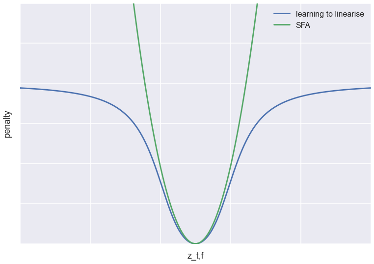
As you can see, both objectives have a minimum at the same location: they both try to force $z_{t,f}$ to linearly interpolate between the neighbouring timesteps. However, while SFA has a quadratic penalty, the learning to linearise objective tapers off at long distances. Compare this to Tukey's loss function used in outlier-resistant robust regression.

Based on this, my prediction is that compared to SFA, this loss function is more tolerant of outliers, which in the temporal domain would mean abrupt jumps in the latent representation. So while SFA is equivalent to assuming that the latent features follow a Brownian-motion-like Ornstein–Uhlenbeck process, I'd imagine this prior corresponds to something like a jump diffusion process (although I don't think the analogy holds mathematically).

Which one of these inductive biases/priors are better at exploiting temporal information in natural video? Slow Brownian motion, or nearly-linear trajectories with potentially a few jumps Unfortunately, don't expect any empirical answer to that from the paper. All experiments seem to be performed on artificially constructed examples, where the temporal information is synthetically engineered. Nor there is any real comparison to SFA.

#### Representing predictive uncertainty with auxillary variables

While the encoder network learns to construct smoothly varrying features $z_t$, the model also has a decoder network that tries to reconstruct $x_t$ and predict subsequent frames. This, the authors agree, is necessary in order for $z_t$ to contain enough relevant information about the frame $x_t$ (more about whether or not this is necessary later). The precise way this decoding is done has a novel idea as well: minimising over auxillary variables.

Let's say our task is to predict a future frame $x_{t+k}$ based on the latent representation $z_{t}$. The problem is, this is a very hard problem. In video, just like in real life, anything can happen. Imagine you're modelling soccer footage, and the ball is about to hit the goalpost. In order to predict the next frames, not only do we have to know about natural image statistics, we also have to be able to predict whether the goal is in or not. An optimal predictive model would give a highly multimodal probability distribution as its answer. If you use the L2 loss with a deterministic feed-forward predictive network, it's likely to come up with a very blurry image, which would correspont to the average of this nasty multimodal distribution. This calls for something better, either a smarter objective function, or a better way of representing predictive uncertainty.

The solution the authors gave is to introduce hidden variables $\delta_{t}$, that the decoder network also receives as input in addition to $z_t$. For each frame, $\delta_t$ is optimised so that only the best possible reconstruction is taken into account in the loss function. Thus, the decoder network is allowed to use $\delta$ as a source of non-determinism to hedge its bets as to what the contents of the next frame will be. This is one step closer to the ideal setting where the decoder network is allowed to give a full probability distribution of possibilities and then is evaluated using a strictly proper scoring rule.

This inner loop minimisation (of $\delta$) looks very tedious, and introduces a few more parameters that may be hard to set. The algorithm is reminiscent of the E-step in expectation-maximisation, and also very similar to the iterated closest point algorithm Andrew Fitzgibbon talked about in his tutorial at BMVC this year.

In his tutorial, Andrew gave examples where jointly optimising model parameters and auxiliary variables ($\delta$) is advantageous, and I think the same logic applies here. Instead of the inner loop, simultaneous optimisation helps fixing some pathologies, like slow convergence near the optimum. In addition, Andrew advocates exploiting the sparsity structure of the Hessian to implement efficient second-order gradient-based optimisation methods. These tricks are explained in paragraphs around equation 8 in (Prasad et al, 2010).

#### Predictive model: Is it necessary?

On a more fundamental level, I question whether the predictive decoder network is really a necessary addition to make L2L work.

The authors observe that the objective function is minimised by the "trivial" solutions $z_{t} = at + b$, where $a,b$ can be arbitrary constants. They then say that in order to make sure features do something more than just discover some of these trivial solutions, we also have to include a decoder network, that uses $z_t$ to predict future frames. I believe this is not necessary at all.

Because $z_t$ is a deterministic function of $x_t$, and $t$ is not accessible to $z_{t}$ in any other way than through inferring it from $x_t$, as long as $a\neq 0$, the linear solutions are not trivial at all. If the network discovers $z_{t} = at, a\neq 0$, you should in fact be very happy (assuming a single feature). The only problems with trivial solutions occur when $z_{t} = b$ ($z$ doesn't depend on the data at all) or when $z$ is multidimensional and several redundant features are sensitive to exactly the same thing.

These trivial solutions could be avoided the same way they are avoided in SFA, by constraining the overall spatial covariance of $z_{t}$ over the videoclip to be $I$. This would force each feature to vary at least a little bit with data- hence avoiding the trivial constant solutions. It would also force features to be linearly decorrelated - solving the redundant features problem.

So I wonder if the decoder network is indeed a necessary addition to the model. I would love to encourage the authors to implement their new hypothesis of a prior both with and without the decoder. They may already have tried it without and found it really didn’t work, so it might just be a matter of including those results. This would in turn allow us to see SFA and L2L side-by-side, and learn something about whether and why their prior is better than the sl

This post is a comment on the Laplacian pyramid-based generative model proposed by researchers from NYU/Facebook AI Research.

Let me start by saying that I really like this model, and I think - looking at the samples drawn - it represents a nice big step towards convincing generative models of natural images.

To summarise the model, the authors use the Laplacian pyramid representation of images, where you recursively decompose the image to a lower resolution subsampled component and the high-frequency residual. The reason this decomposition is favoured in image processing is the fact that the high-frequency residuals tend to be very sparse, so they are relatively easy to compress and encode.

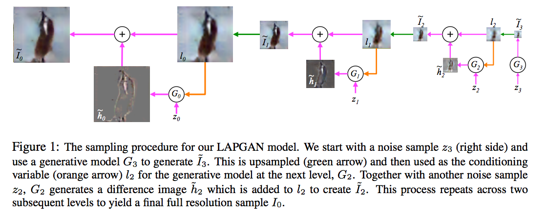
In this paper the authors propose using convolutional neural networks at each layer of the Laplacian pyramid representation to generate an image sequentially, increasing the resolution at each step. The convnet at each layer is conditioned on the lower resolution image, and some noise component $z_k$, and generates a random higher resolution image. The process continues recursively until the desired resilution is reached. For training they use the adversarial objective function. Below is the main figure that explains how the generative model works, I encourage everyone to have a look at the paper for more details:

![](http://www.inference.vc/content/images/2015/07/Screen-Shot-2015-07-23-at-11-15-17.png)

#### An argument about Conditional Entropies

What I think is weird about the model is the precise amount of noise that is injected at each layer/resolution. In the schematic above, these are the $z_k$ variables. Adding the noise is crucial to defining a probabilistic generative process; this is how it defines a probability distribution.

I think it's useful to think about entropies of natural images at different resolutions. When doing generative modelling or unsuperised learning, we want to capture the distribution of data. One important aspect of a probability distribution is its entropy, which measures the variability of the random quantity. In this case, we want to describe the statistics of the full resolution observed natural image $I_0$. (I borrow the authors' notation where $I_0$ represents the highest resolution image, and $I_k$ represent the $k$-times subsampled version. Using the Laplacian pyramid representation, we can decompose the entropy of an image in the following way:

$$\mathbb{H}[I_0] = \mathbb{H}[I_{K}] + \sum_{k=0}^{K-1} \mathbb{H}[I_k\vert I_{k+1}].$$

The reason why the above decomposition holds is very simple. Because $I_{k+1}$ is a deterministic function of $I_{k}$ (subsampling), the conditional entropy $\mathbb{H}[I_{k+1}\vert I_{k}] = 0$. Therefore the joint entropy of the two variables is simply the entropy of the higher resolution image $I_{k}$, that is $\mathbb{H}[I_{k},I_{k+1}] = \mathbb{H}[I_{k}] + \mathbb{H}[I_{k+1}\vert I_{k}] = \mathbb{H}[I_{k}]$. So by induction, the join entropy of all images $I_{k}$ is just the marginal entropy of the highest resolution image $I_0$. Applying the chain rule for joint entropies we get the expression above.

Now, the interesting bit is how the conditional entropies $\mathbb{H}[I_k\vert I_{k+1}]$ are 'achieved' in the Laplacian pyramid generative model paper. These entropies are provided by the injected random noise variables $z_k$. By the information processing lemma $\mathbb{H}[I_k\vert I_{k+1}] \leq \mathbb{H}[z_k]$. The authors choose $z_k$ to be uniform random variables whose dimensionality grows with the resolution of $I_k$. To quote them "The noise input $z_k$ to $G_k$ is presented as a 4th color plane to low-pass $l_k$, hence its dimensionality varies with the pyramid level." Therefore $\mathbb{H}[z_k] \propto 4^{-k}$, assuming that the pixel count quadruples at each layer.

So the conditional entropy $\mathbb{H}[I_k\vert I_{k+1}]$ is allowed to grow exponentially with resolution, at the same rate it would grow if the images contained pure white noise. In their model, they allow the per-pixel conditional entropy $c\cdot 4^{-k}\cdot \mathbb{H}[I_k\vert I_{k+1}]$ to be constant across resolutions. To me, this seems undesirable. My intuition is, for natural images, $\mathbb{H}[I_k\vert I_{k+1}]$ may grow as $k$ decreases (because the dimensionality gorws), but the per-pixel value $c\cdot 4^{k}\cdot \mathbb{H}[I_k\vert I_{k+1}]$ should decrease or converge to $0$ as the resolution increases. Very low low-resolution subsampled natural images behave a little bit like white noise, there is a lot of variability in them. But as you increase the resolution, the probability distribution of the high-res image given the low-res image will become a lot sharper.

In terms of model capacity, this is not a problem, inasmuch as the convolutional models $G_{k}$ can choose to ignore some variance in $z_k$ and learn a more deterministic superresolution process. However, adding unnecessarily high entropy will almost certainly make the fitting of such model harder. For example, the adversarial training process relies on sampling from $z_k$, and the procedure is pretty sensitive to sampling noise. If you make the distribution of $z_k$ unneccessarily high entropy, you will end up doing a lot of extra work during training until the network figures out to ignore the extra variance.

To solve this problem, I propose to keep the entropy of the noise vectors constant, or make them grow sub-linearly with the number of pixels in the image. This mperhaps akes the generative convnets harder to implement. Another quick solution would be to introduce dependence between components of $z_k$ via a low-rank covariance matrix, or some sort of a hashing trick.

#### Adversarial training vs superresolution autoencoders

Another weird thing is that the adversarial objective function forgets the identity of the image. For example, you would want your model so that

`"if at the previous layer you have a low-resolution parrot, the next layer should be a higher-resolution parrot"`

Instead, what you get with the adversarial objective is

`"if at the previous layer you have a low-resolution parrot, the next layer should output a higher-dimensional image that looks like a plausible natural image"`

So, there is nothing in the objective function that enforces dependency between subsequent layers of the pyramid. I think if you made $G_k$ very complex, it could just learn to model natural images by itself, so that $I_{k}$ is in essence independent of $I_{k+1}$ and is purely driven by the noise $z_{k}$. You could sidestep this problem by restricting the complexity of the generative nets, or, again, to restrict the entropy of the noise.

Overall, I think the approach would benefit from a combination of the adversarial and a supervised (superresolution autoencoder) objective function.