* They present a variation of Faster R-CNN.
    * Faster R-CNN is a model that detects bounding boxes in images.
  * Their variation is about as accurate as the best performing versions of Faster R-CNN.
  * Their variation is significantly faster than these variations (roughly 50ms per image).

### How
  * PVANET reuses the standard Faster R-CNN architecture:
    * A base network that transforms an image into a feature map.
    * A region proposal network (RPN) that uses the feature map to predict bounding box candidates.
    * A classifier that uses the feature map and the bounding box candidates to predict the final bounding boxes.
  * PVANET modifies the base network and keeps the RPN and classifier the same.
  * Inception
    * Their base network uses eight Inception modules.
    * They argue that these are good choices here, because they are able to represent an image at different scales (aka at different receptive field sizes)
      due to their mixture of 3x3 and 1x1 convolutions.
      * ![Receptive field sizes in inception modules](images/PVANET__inception_fieldsize.jpg?raw=true "Receptive field sizes in inception modules")
    * Representing an image at different scales is useful here in order to detect both large and small bounding boxes.
    * Inception modules are also reasonably fast.
    * Visualization of their Inception modules:
      * ![Inception modules architecture](images/PVANET__inception_modules.jpg?raw=true "Inception modules architecture")
  * Concatenated ReLUs
    * Before the eight Inception modules, they start the network with eight convolutions using concatenated ReLUs.
    * These CReLUs compute both the classic ReLU result (`max(0, x)`) and concatenate to that the negated result, i.e. something like `f(x) = max(0, x <concat> (-1)*x)`.
    * That is done, because among the early one can often find pairs of convolution filters that are the negated variations of each other.
      So by adding CReLUs, the network does not have to compute these any more, instead they are created (almost) for free, reducing the computation time by up to 50%.
    * Visualization of their final CReLU block:
      * TODO
      * ![CReLU modules](https://raw.githubusercontent.com/aleju/papers/master/neural-nets/images/PVANET__crelu.jpg?raw=true "CReLU modules")
  * Multi-Scale output
    * Usually one would generate the final feature map simply from the output of the last convolution.
    * They instead combine the outputs of three different convolutions, each resembling a different scale (or level of abstraction).
    * They take one from an early point of the network (downscaled), one from the middle part (kept the same) and one from the end (upscaled).
    * They concatenate these and apply a 1x1 convolution to generate the final output.
  * Other stuff
    * Most of their network uses residual connections (including the Inception modules) to facilitate learning.
    * They pretrain on ILSVRC2012 and then perform fine-tuning on MSCOCO, VOC 2007 and VOC 2012.
    * They use plateau detection for their learning rate, i.e. if a moving average of the loss does not improve any more, they decrease the learning rate. They say that this increases accuracy significantly.
    * The classifier in Faster R-CNN consists of fully connected layers. They compress these via Truncated SVD to speed things up. (That was already part of Fast R-CNN, I think.)

### Results
  * On Pascal VOC 2012 they achieve 82.5% mAP at 46ms/image (Titan X GPU).
    * Faster R-CNN + ResNet-101: 83.8% at 2.2s/image.
    * Faster R-CNN + VGG16: 75.9% at 110ms/image.
    * R-FCN + ResNet-101: 82.0% at 133ms/image.
  * Decreasing the number of region proposals from 300 per image to 50 almost doubles the speed (to 27ms/image) at a small loss of 1.5 percentage points mAP.
  * Using Truncated SVD for the classifier reduces the required timer per image by about 30% at roughly 1 percentage point of mAP loss.

  * They present a variation of Faster R-CNN, i.e. a model that predicts bounding boxes in images and classifies them.
  * In contrast to Faster R-CNN, their model is fully convolutional.
  * In contrast to Faster R-CNN, the computation per bounding box candidate (region proposal) is very low.

### How
  * The basic architecture is the same as in Faster R-CNN:
    * A base network transforms an image to a feature map. Here they use ResNet-101 to do that.
    * A region proposal network (RPN) uses the feature map to locate bounding box candidates ("region proposals") in the image.
    * A classifier uses the feature map and the bounding box candidates and classifies each one of them into `C+1` classes,
      where `C` is the number of object classes to spot (e.g. "person", "chair", "bottle", ...) and `1` is added for the background.
      * During that process, small subregions of the feature maps (those that match the bounding box candidates) must be extracted and converted to fixed-sizes matrices.
        The method to do that is called "Region of Interest Pooling" (RoI-Pooling) and is based on max pooling.
        It is mostly the same as in Faster R-CNN.
    * Visualization of the basic architecture:
      * ![Architecture](https://raw.githubusercontent.com/aleju/papers/master/neural-nets/images/R-FCN__architecture.jpg?raw=true "Architecture")
  * Position-sensitive classification
    * Fully convolutional bounding box detectors tend to not work well.
    * The authors argue, that the problems come from the translation-invariance of convolutions, which is a desirable property in the case of classification but not when precise localization of objects is required.
    * They tackle that problem by generating multiple heatmaps per object class, each one being slightly shifted ("position-sensitive score maps").
    * More precisely:
      * The classifier generates per object class `c` a total of `k*k` heatmaps.
      * In the simplest form `k` is equal to `1`. Then only one heatmap is generated, which signals whether a pixel is part of an object of class `c`.
      * They use `k=3*3`. The first of those heatmaps signals, whether a pixel is part of the *top left* corner of a bounding box of class `c`. The second heatmap signals, whether a pixel is part of the *top center* of a bounding box of class `c` (and so on).
      * The RoI-Pooling is applied to these heatmaps.
      * For `k=3*3`, each bounding box candidate is converted to `3*3` values. The first one resembles the top left corner of the bounding box candidate. Its value is generated by taking the average of the values in that area in the first heatmap.
      * Once the `3*3` values are generated, the final score of class `c` for that bounding box candidate is computed by averaging the values.
      * That process is repeated for all classes and a softmax is used to determine the final class.
      * The graphic below shows examples for that:
        * ![Architecture](https://raw.githubusercontent.com/aleju/papers/master/neural-nets/images/R-FCN__examples.jpg?raw=true "Examples")
    * The above described RoI-Pooling uses only averages and hence is almost (computationally) free.
      * They make use of that during the training by sampling many candidates and only backpropagating on those with high losses (online hard example mining, OHEM).
  * À trous trick
    * In order to increase accuracy for small bounding boxes they use the à trous trick.
    * That means that they use a pretrained base network (here ResNet-101), then remove a pooling layer and set the à trous rate (aka dilation) of all convolutions after the removed pooling layer to `2`.
      * The á trous rate describes the distance of sampling locations of a convolution. Usually that is `1` (sampled locations are right next to each other). If it is set to `2`, there is one value "skipped" between each pair of neighbouring sampling location.
    * By doing that, the convolutions still behave as if the pooling layer existed (and therefore their weights can be reused). At the same time, they work at an increased resolution, making them more capable of classifying small objects. (Runtime increases though.)
  * Training of R-FCN happens similarly to Faster R-CNN.

### Results
  * Similar accuracy as the most accurate Faster R-CNN configurations at a lower runtime of roughly 170ms per image.
  * Switching to ResNet-50 decreases accuracy by about 2 percentage points mAP (at faster runtime). Switching to ResNet-152 seems to provide no measureable benefit.
  * OHEM improves mAP by roughly 2 percentage points.
  * À trous trick improves mAP by roughly 2 percentage points.
  * Training on `k=1` (one heatmap per class) results in a failure, i.e. a model that fails to predict bounding boxes. `k=7` is slightly more accurate than `k=3`.

* R-CNN and its successor Fast R-CNN both rely on a "classical" method to find region proposals in images (i.e. "Which regions of the image look like they *might* be objects?").
  * That classical method is selective search.
  * Selective search is quite slow (about two seconds per image) and hence the bottleneck in Fast R-CNN.
  * They replace it with a neural network (region proposal network, aka RPN).
  * The RPN reuses the same features used for the remainder of the Fast R-CNN network, making the region proposal step almost free (about 10ms).

### How
  * They now have three components in their network:
    * A model for feature extraction, called the "feature extraction network" (**FEN**). Initialized with the weights of a pretrained network (e.g. VGG16).
    * A model to use these features and generate region proposals, called the "Region Proposal Network" (**RPN**).
    * A model to use these features and region proposals to classify each regions proposal's object and readjust the bounding box, called the "classification network" (**CN**). Initialized with the weights of a pretrained network (e.g. VGG16).
    * Usually, FEN will contain the convolutional layers of the pretrained model (e.g. VGG16), while CN will contain the fully connected layers.
    * (Note: Only "RPN" really pops up in the paper, the other two remain more or less unnamed. I added the two names to simplify the description.)
    * Rough architecture outline:
      * ![Architecture](images/Faster_R-CNN__architecture.jpg?raw=true "Architecture")
  * The basic method at test is as follows:
    1. Use FEN to convert the image to features.
    2. Apply RPN to the features to generate region proposals.
    3. Use Region of Interest Pooling (RoI-Pooling) to convert the features of each region proposal to a fixed sized vector.
    4. Apply CN to the RoI-vectors to a) predict the class of each object (out of `K` object classes and `1` background class) and b) readjust the bounding box dimensions (top left coordinate, height, width).
  * RPN
    * Basic idea:
      * Place anchor points on the image, all with the same distance to each other (regular grid).
      * Around each anchor point, extract rectangular image areas in various shapes and sizes ("anchor boxes"), e.g. thin/square/wide and small/medium/large rectangles. (More precisely: The features of these areas are extracted.)
      * Visualization:
        * ![Anchor Boxes](https://raw.githubusercontent.com/aleju/papers/master/neural-nets/images/Faster_R-CNN__anchor_boxes.jpg?raw=true "Anchor Boxes")
      * Feed the features of these areas through a classifier and let it rate/predict the "regionness" of the rectangle in a range between 0 and 1. Values greater than 0.5 mean that the classifier thinks the rectangle might be a bounding box. (CN has to analyze that further.)
      * Feed the features of these areas through a regressor and let it optimize the region size (top left coordinate, height, width). That way you get all kinds of possible bounding box shapes, even though you only use a few base shapes.
    * Implementation:
      * The regular grid of anchor points naturally arises due to the downscaling of the FEN, it doesn't have to be implemented explicitly.
      * The extraction of anchor boxes and classification + regression can be efficiently implemented using convolutions.
        * They first apply a 3x3 convolution on the feature maps. Note that the convolution covers a large image area due to the downscaling.
          * Not so clear, but sounds like they use 256 filters/kernels for that convolution.
        * Then they apply some 1x1 convolutions for the classification and regression.
          * They use `2*k` 1x1 convolutions for classification and `4*k` 1x1 convolutions for regression, where `k` is the number of different shapes of anchor boxes.
      * They use `k=9` anchor box types: Three sizes (small, medium, large), each in three shapes (thin, square, wide).
      * The way they build training examples (below) forces some 1x1 convolutions to react only to some anchor box types.
    * Training:
      * Positive examples are anchor boxes that have an IoU with a ground truth bounding box of 0.7 or more. If no anchor point has such an IoU with a specific box, the one with the highest IoU is used instead.
      * Negative examples are all anchor boxes that have IoU that do not exceed 0.3 for any bounding box.
      * Any anchor point that falls in neither of these groups does not contribute to the loss.
      * Anchor boxes that would violate image boundaries are not used as examples.
      * The loss is similar to the one in Fast R-CNN: A sum consisting of log loss for the classifier and smooth L1 loss (=smoother absolute distance) for regression.
      * Per batch they only sample examples from one image (for efficiency).
      * They use 128 positive examples and 128 negative ones. If they can't come up with 128 positive examples, they add more negative ones.
    * Test:
      * They use non-maximum suppression (NMS) to remove too identical region proposals, i.e. among all region proposals that have an IoU overlap of 0.7 or more, they pick the one that has highest score.
      * They use the 300 proposals with highest score after NMS (or less if there aren't that many).
  * Feature sharing
    * They want to share the features of the FEN between the RPN and the CN.
    * So they need a special training method that fine-tunes all three components while keeping the features extracted by FEN useful for both RPN and CN at the same time (not only for one of them).
    * Their training methods are:
      * Alternating traing: One batch for FEN+RPN, one batch for FEN+CN, then again one batch for FEN+RPN and so on.
      * Approximate joint training: Train one network of FEN+RPN+CN. Merge the gradients of RPN and CN that arrive at FEN via simple summation. This method does not compute a gradient from CN through the RPN's regression task, as that is non-trivial. (This runs 25-50% faster than alternating training, accuracy is mostly the same.)
      * Non-approximate joint training: This would compute the above mentioned missing gradient, but isn't implemented.
      * 4-step alternating training:
        1. Clone FEN to FEN1 and FEN2.
        2. Train the pair FEN1 + RPN.
        3. Train the pair FEN2 + CN using the region proposals from the trained RPN.
        4. Fine-tune the pair FEN2 + RPN. FEN2 is fixed, RPN takes the weights from step 2.
        5. Fine-tune the pair FEN2 + CN. FEN2 is fixed, CN takes the weights from step 3, region proposals come from RPN from step 4.

* Results
  * Example images:
    * ![Example images](https://raw.githubusercontent.com/aleju/papers/master/neural-nets/images/Faster_R-CNN__examples.jpg?raw=true "Example images")
  * Pascal VOC (with VGG16 as FEN)
    * Using an RPN instead of SS (selective search) slightly improved mAP from 66.9% to 69.9%.
    * Training RPN and CN on the same FEN (sharing FEN's weights) does not worsen the mAP, but instead improves it slightly from 68.5% to 69.9%.
  * Using the RPN instead of SS significantly speeds up the network, from 1830ms/image (less than 0.5fps) to 198ms/image (5fps). (Both stats with VGG16. They also use ZF as the FEN, which puts them at 17fps, but mAP is lower.)
  * Using per anchor point more scales and shapes (ratios) for the anchor boxes improves results.
    * 1 scale, 1 ratio: 65.8% mAP (scale `128*128`, ratio 1:1) or 66.7% mAP (scale `256*256`, same ratio).
    * 3 scales, 3 ratios: 69.9% mAP (scales `128*128`, `256*256`, `512*512`; ratios 1:1, 1:2, 2:1).
  * Two-staged vs one-staged
    * Instead of the two-stage system (first, generate proposals via RPN, then classify them via CN), they try a one-staged system.
    * In the one-staged system they move a sliding window over the computed feature maps and regress at every location the bounding box sizes and classify the box.
    * When doing this, their performance drops from 58.7% to about 54%.

  * The original R-CNN had three major disadvantages:
    1. Two-staged training pipeline: Instead of only training a CNN, one had to train first a CNN and then multiple SVMs.
    2. Expensive training: Training was slow and required lots of disk space (feature vectors needed to be written to disk for all region proposals (2000 per image) before training the SVMs).
    3. Slow test: Each region proposal had to be handled independently.
  * Fast R-CNN ist an improved version of R-CNN and tackles the mentioned problems.
    * It no longer uses SVMs, only CNNs (single-stage).
    * It does one single feature extraction per image instead of per region, making it much faster (9x faster at training, 213x faster at test).
    * It is more accurate than R-CNN.

### How
  * The basic architecture, training and testing methods are mostly copied from R-CNN.
  * For each image at test time they do:
    * They generate region proposals via selective search.
    * They feed the image once through the convolutional layers of a pre-trained network, usually VGG16.
    * For each region proposal they extract the respective region from the features generated by the network.
    * The regions can have different sizes, but the following steps need fixed size vectors. So each region is downscaled via max-pooling so that it has a size of 7x7 (so apparently they ignore regions of sizes below 7x7...?).
      * This is called Region of Interest Pooling (RoI-Pooling).
      * During the backwards pass, partial derivatives can be transferred to the maximum value (as usually in max pooling). That derivative values are summed up over different regions (in the same image).
    * They reshape the 7x7 regions to vectors of length `F*7*7`, where `F` was the number of filters in the last convolutional layer.
    * They feed these vectors through another network which predicts:
      1. The class of the region (including background class).
      2. Top left x-coordinate, top left y-coordinate, log height and log width of the bounding box (i.e. it fine-tunes the region proposal's bounding box). These values are predicted once for every class (so `K*4` values).
  * Architecture as image:
    * ![Architecture](https://raw.githubusercontent.com/aleju/papers/master/neural-nets/images/Fast_R-CNN__architecture.jpg?raw=true "Architecture")
  * Sampling for training
    * Efficiency
      * If batch size is `B` it is inefficient to sample regions proposals from `B` images as each image will require a full forward pass through the base network (e.g. VGG16).
      * It is much more efficient to use few images to share most of the computation between region proposals.
      * They use two images per batch (each 64 region proposals) during training.
      * This technique introduces correlations between examples in batches, but they did not observe any problems from that.
      * They call this technique "hierarchical sampling" (first images, then region proposals).
    * IoUs
      * Positive examples for specific classes during training are region proposals that have an IoU with ground truth bounding boxes of `>=0.5`.
      * Examples for background region proposals during training have IoUs with any ground truth box in the interval `(0.1, 0.5]`.
        * Not picking IoUs below 0.1 is similar to hard negative mining.
    * They use 25% positive examples, 75% negative/background examples per batch.
    * They apply horizontal flipping as data augmentation, nothing else.
  * Outputs
    * For their class predictions the use a simple softmax with negative log likelihood.
    * For their bounding box regression they use a smooth L1 loss (similar to mean absolute error, but switches to mean squared error for very low values).
      * Smooth L1 loss is less sensitive to outliers and less likely to suffer from exploding gradients.
    * The smooth L1 loss is only active for positive examples (not background examples). (Not active means that it is zero.)
  * Training schedule
    * The use SGD.
    * They train 30k batches with learning rate 0.001, then 0.0001 for another 10k batches. (On Pascal VOC, they use more batches on larger datasets.)
    * They use twice the learning rate for the biases.
    * They use momentum of 0.9.
    * They use parameter decay of 0.0005.
  * Truncated SVD
    * The final network for class prediction and bounding box regression has to be applied to every region proposal.
    * It contains one large fully connected hidden layer and one fully connected output layer (`K+1` classes plus `K*4` regression values).
    * For 2000 proposals that becomes slow.
    * So they compress the layers after training to less weights via truncated SVD.
      * A weights matrix is approximated via ![T-SVD equation](https://raw.githubusercontent.com/aleju/papers/master/neural-nets/images/Fast_R-CNN__tsvd.jpg?raw=true "T-SVD equation")
        * U (`u x t`) are the first `t` left-singular vectors of W.
        * Sigma is a `t x t` diagonal matrix of the top `t` singular values.
        * V (`v x t`) are the first `t` right-singular vectors of W.
      * W is then replaced by two layers: One contains `Sigma V^T` as weights (no biases), the other contains `U` as weights (with original biases).
      * Parameter count goes down to `t(u+v)` from `uv`.

### Results
  * They try three base models:
    * AlexNet (Small, S)
    * VGG-CNN-M-1024 (Medium, M)
    * VGG16 (Large, L)
  * On VGG16 and Pascal VOC 2007, compared to original R-CNN:
    * Training time down to 9.5h from 84h (8.8x faster).
    * Test rate *with SVD* (1024 singular values) improves from 47 seconds per image to 0.22 seconds per image (213x faster).
    * Test rate *without SVD* improves similarly to 0.32 seconds per image.
    * mAP improves from 66.0% to 66.6% (66.9% without SVD).
    * Per class accuracy results:
      * Fast_R-CNN__pvoc2012.jpg
      * ![VOC2012 results](https://raw.githubusercontent.com/aleju/papers/master/neural-nets/images/Fast_R-CNN__pvoc2012.jpg?raw=true "VOC2012 results")
  * Fixing the weights of VGG16's convolutional layers and only fine-tuning the fully connected layers (those are applied to each region proposal), decreases the accuracy to 61.4%.
    * This decrease in accuracy is most significant for the later convolutional layers, but marginal for the first layers.
    * Therefor they only train the convolutional layers starting with `conv3_1` (9 out of 13 layers), which speeds up training.
  * Multi-task training
    * Training models on classification and bounding box regression instead of only on classification improves the mAP (from 62.6% to 66.9%).
    * Doing this in one hierarchy instead of two seperate models (one for classification, one for bounding box regression) increases mAP by roughly 2-3 percentage points.
  * They did not find a significant benefit of training the model on multiple scales (e.g. same image sometimes at 400x400, sometimes at 600x600, sometimes at 800x800 etc.).
    * Note that their raw CNN (everything before RoI-Pooling) is fully convolutional, so they can feed the images at any scale through the network.
  * Increasing the amount of training data seemed to improve mAP a bit, but not as much as one might hope for.
  * Using a softmax loss instead of an SVM seemed to marginally increase mAP (0-1 percentage points).
  * Using more region proposals from selective search does not simply increase mAP. Instead it can lead to higher recall, but lower precision.
    * ![Proposal schemes](https://raw.githubusercontent.com/aleju/papers/master/neural-nets/images/Fast_R-CNN__proposal_schemes.jpg?raw=true "Proposal schemes")
  * Using densely sampled region proposals (as in sliding window) significantly reduces mAP (from 59.2% to 52.9%). If SVMs instead of softmaxes are used, the results are even worse (49.3%).

  * Previously, methods to detect bounding boxes in images were often based on the combination of manual feature extraction with SVMs.
  * They replace the manual feature extraction with a CNN, leading to significantly higher accuracy.
  * They use supervised pre-training on auxiliary datasets to deal with the small amount of labeled data (instead of the sometimes used unsupervised pre-training).
  * They call their method R-CNN ("Regions with CNN features").

### How
  * Their system has three modules: 1) Region proposal generation, 2) CNN-based feature extraction per region proposal, 3) classification.
    * ![Architecture](https://raw.githubusercontent.com/aleju/papers/master/neural-nets/images/Rich_feature_hierarchies_for_accurate_object_detection_and_semantic_segmentation__architecture.jpg?raw=true "Architecture")
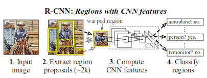
  * Region proposals generation
    * A region proposal is a bounding box candidate that *might* contain an object.
    * By default they generate 2000 region proposals per image.
    * They suggest "simple" (i.e. not learned) algorithms for this step (e.g. objectneess, selective search, CPMC).
    * They use selective search (makes it comparable to previous systems).
  * CNN features
    * Uses a CNN to extract features, applied to each region proposal (replaces the previously used manual feature extraction).
    * So each region proposal ist turned into a fixed length vector.
    * They use AlexNet by Krizhevsky et al. as their base CNN (takes 227x227 RGB images, converts them into 4096-dimensional vectors).
    * They add `p=16` pixels to each side of every region proposal, extract the pixels and then simply resize them to 227x227 (ignoring aspect ratio, so images might end up distorted).
    * They generate one 4096d vector per image, which is less than what some previous manual feature extraction methods used. That enables faster classification, less memory usage and thus more possible classes.
  * Classification
    * A classifier that receives the extracted feature vectors (one per region proposal) and classifies them into a predefined set of available classes (e.g. "person", "car", "bike", "background / no object").
    * They use one SVM per available class.
    * The regions that were not classified as background might overlap (multiple bounding boxes on the same object).
      * They use greedy non-maximum suppresion to fix that problem (for each class individually).
      * That method simply rejects regions if they overlap strongly with another region that has higher score.
      * Overlap is determined via Intersection of Union (IoU).
  * Training method
    * Pre-Training of CNN
      * They use AlexNet pretrained on Imagenet (1000 classes).
      * They replace the last fully connected layer with a randomly initialized one that leads to `C+1` classes (`C` object classes, `+1` for background).
    * Fine-Tuning of CNN
      * The use SGD with learning rate `0.001`.
      * Batch size is 128 (32 positive windows, 96 background windows).
      * A region proposal is considered positive, if its IoU with any ground-truth bounding box is `>=0.5`.
    * SVM
      * They train one SVM per class via hard negative mining.
      * For positive examples they use here an IoU threshold of `>=0.3`, which performed better than 0.5.

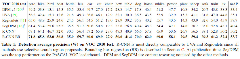
### Results
  * Pascal VOC 2010
    * They: 53.7% mAP
    * Closest competitor (SegDPM): 40.4% mAP
    * Closest competitor that uses the same region proposal method (UVA): 35.1% mAP
    * ![Scores on Pascal VOC 2010](https://raw.githubusercontent.com/aleju/papers/master/neural-nets/images/Rich_feature_hierarchies_for_accurate_object_detection_and_semantic_segmentation__scores.jpg?raw=true "Scores on Pascal VOC 2010")
  * ILSVRC2013 detection
    * They: 31.4% mAP
    * Closest competitor (OverFeat): 24.3% mAP
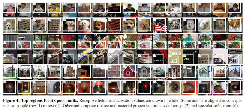
  * The feed a large number of region proposals through the network and log for each filter in the last conv-layer which images activated it the most:
    * ![Activations](https://raw.githubusercontent.com/aleju/papers/master/neural-nets/images/Rich_feature_hierarchies_for_accurate_object_detection_and_semantic_segmentation__activations.jpg?raw=true "Activations")
  * Usefulness of layers:
    * They remove later layers of the network and retrain in order to find out which layers are the most useful ones.
    * Their result is that both fully connected layers of AlexNet seemed to be very domain-specific and profit most from fine-tuning.
  * Using VGG16:
    * Using VGG16 instead of AlexNet increased mAP from 58.5% to 66.0% on Pascal VOC 2007.
    * Computation time was 7 times higher.
  * They train a linear regression model that improves the bounding box dimensions based on the extracted features of the last pooling layer. That improved their mAP by 3-4 percentage points.
  * The region proposals generated by selective search have a recall of 98% on Pascal VOC and 91.6% on ILSVRC2013 (measured by IoU of `>=0.5`).