
|
Welcome to ShortScience.org! |


|
- ShortScience.org is a platform for post-publication discussion aiming to improve accessibility and reproducibility of research ideas.
- The website has 1583 public summaries, mostly in machine learning, written by the community and organized by paper, conference, and year.
- Reading summaries of papers is useful to obtain the perspective and insight of another reader, why they liked or disliked it, and their attempt to demystify complicated sections.
- Also, writing summaries is a good exercise to understand the content of a paper because you are forced to challenge your assumptions when explaining it.
- Finally, you can keep up to date with the flood of research by reading the latest summaries on our Twitter and Facebook pages.
StackGAN: Text to Photo-realistic Image Synthesis with Stacked Generative Adversarial Networks
Zhang, Han and Xu, Tao and Li, Hongsheng and Zhang, Shaoting and Huang, Xiaolei and Wang, Xiaogang and Metaxas, Dimitris N.
arXiv e-Print archive - 2016 via Local Bibsonomy
Keywords: dblp
Zhang, Han and Xu, Tao and Li, Hongsheng and Zhang, Shaoting and Huang, Xiaolei and Wang, Xiaogang and Metaxas, Dimitris N.
arXiv e-Print archive - 2016 via Local Bibsonomy
Keywords: dblp


[link]
* They propose a two-stage GAN architecture that generates 256x256 images of (relatively) high quality.
* The model gets text as an additional input and the images match the text.
### How
* Most of the architecture is the same as in any GAN:
* Generator G generates images.
* Discriminator D discriminates betweens fake and real images.
* G gets a noise variable `z`, so that it doesn't always do the same thing.
* Two-staged image generation:
* Instead of one step, as in most GANs, they use two steps, each consisting of a G and D.
* The first generator creates 64x64 images via upsampling.
* The first discriminator judges these images via downsampling convolutions.
* The second generator takes the image from the first generator, downsamples it via convolutions, then applies some residual convolutions and then re-upsamples it to 256x256.
* The second discriminator is comparable to the first one (downsampling convolutions).
* Note that the second generator does not get an additional noise term `z`, only the first one gets it.
* For upsampling, they use 3x3 convolutions with ReLUs, BN and nearest neighbour upsampling.
* For downsampling, they use 4x4 convolutions with stride 2, Leaky ReLUs and BN (the first convolution doesn't seem to use BN).
* Text embedding:
* The generated images are supposed to match input texts.
* These input texts are embedded to vectors.
* These vectors are added as:
1. An additional input to the first generator.
2. An additional input to the second generator (concatenated after the downsampling and before the residual convolutions).
3. An additional input to the first discriminator (concatenated after the downsampling).
4. An additional input to the second discriminator (concatenated after the downsampling).
* In case the text embeddings need to be matrices, the values are simply reshaped to `(N, 1, 1)` and then repeated to `(N, H, W)`.
* The texts are converted to embeddings via a network at the start of the model.
* Input to that vector: Unclear. (Concatenated word vectors? Seems to not be described in the text.)
* The input is transformed to a vector via a fully connected layer (the text model is apparently not recurrent).
* The vector is transformed via fully connected layers to a mean vector and a sigma vector.
* These are then interpreted as normal distributions, from which the final output vector is sampled. This uses the reparameterization trick, similar to the method in VAEs.
* Just like in VAEs, a KL-divergence term is added to the loss, which prevents each single normal distribution from deviating too far from the unit normal distribution `N(0,1)`.
* The authors argue, that using the VAE-like formulation -- instead of directly predicting an output vector (via FC layers) -- compensated for the lack of labels (smoother manifold).
* Note: This way of generating text embeddings seems very simple. (No recurrence, only about two layers.) It probably won't do much more than just roughly checking for the existence of specific words and word combinations (e.g. "red head").
* Visualization of the architecture:
* 
### Results
* Note: No example images of the two-stage architecture for LSUN bedrooms.
* Using only the first stage of the architecture (first G and D) reduces the Inception score significantly.
* Adding the text to both the first and second generator improves the Inception score slightly.
* Adding the VAE-like text embedding generation (as opposed to only FC layers) improves the Inception score slightly.
* Generating images at higher resolution (256x256 instead of 128x128) improves the Inception score significantly
* Note: The 256x256 architecture has more residual convolutions than the 128x128 one.
* Note: The 128x128 and the 256x256 are both upscaled to 299x299 images before computing the Inception score. That should make the 128x128 images quite blurry and hence of low quality.
* Example images, with text and stage 1/2 results:
* 
* More examples of birds:
* 
* Examples of failures:
* 
* The authors argue, that most failure cases happen when stage 1 messes up.
 |

Self-Normalizing Neural Networks
Günter Klambauer and Thomas Unterthiner and Andreas Mayr and Sepp Hochreiter
arXiv e-Print archive - 2017 via Local arXiv
Keywords: cs.LG, stat.ML
First published: 2017/06/08 (9 years ago)
Abstract: Deep Learning has revolutionized vision via convolutional neural networks (CNNs) and natural language processing via recurrent neural networks (RNNs). However, success stories of Deep Learning with standard feed-forward neural networks (FNNs) are rare. FNNs that perform well are typically shallow and, therefore cannot exploit many levels of abstract representations. We introduce self-normalizing neural networks (SNNs) to enable high-level abstract representations. While batch normalization requires explicit normalization, neuron activations of SNNs automatically converge towards zero mean and unit variance. The activation function of SNNs are "scaled exponential linear units" (SELUs), which induce self-normalizing properties. Using the Banach fixed-point theorem, we prove that activations close to zero mean and unit variance that are propagated through many network layers will converge towards zero mean and unit variance -- even under the presence of noise and perturbations. This convergence property of SNNs allows to (1) train deep networks with many layers, (2) employ strong regularization, and (3) to make learning highly robust. Furthermore, for activations not close to unit variance, we prove an upper and lower bound on the variance, thus, vanishing and exploding gradients are impossible. We compared SNNs on (a) 121 tasks from the UCI machine learning repository, on (b) drug discovery benchmarks, and on (c) astronomy tasks with standard FNNs and other machine learning methods such as random forests and support vector machines. SNNs significantly outperformed all competing FNN methods at 121 UCI tasks, outperformed all competing methods at the Tox21 dataset, and set a new record at an astronomy data set. The winning SNN architectures are often very deep. Implementations are available at: github.com/bioinf-jku/SNNs.
more
less
Günter Klambauer and Thomas Unterthiner and Andreas Mayr and Sepp Hochreiter
arXiv e-Print archive - 2017 via Local arXiv
Keywords: cs.LG, stat.ML
First published: 2017/06/08 (9 years ago)
Abstract: Deep Learning has revolutionized vision via convolutional neural networks (CNNs) and natural language processing via recurrent neural networks (RNNs). However, success stories of Deep Learning with standard feed-forward neural networks (FNNs) are rare. FNNs that perform well are typically shallow and, therefore cannot exploit many levels of abstract representations. We introduce self-normalizing neural networks (SNNs) to enable high-level abstract representations. While batch normalization requires explicit normalization, neuron activations of SNNs automatically converge towards zero mean and unit variance. The activation function of SNNs are "scaled exponential linear units" (SELUs), which induce self-normalizing properties. Using the Banach fixed-point theorem, we prove that activations close to zero mean and unit variance that are propagated through many network layers will converge towards zero mean and unit variance -- even under the presence of noise and perturbations. This convergence property of SNNs allows to (1) train deep networks with many layers, (2) employ strong regularization, and (3) to make learning highly robust. Furthermore, for activations not close to unit variance, we prove an upper and lower bound on the variance, thus, vanishing and exploding gradients are impossible. We compared SNNs on (a) 121 tasks from the UCI machine learning repository, on (b) drug discovery benchmarks, and on (c) astronomy tasks with standard FNNs and other machine learning methods such as random forests and support vector machines. SNNs significantly outperformed all competing FNN methods at 121 UCI tasks, outperformed all competing methods at the Tox21 dataset, and set a new record at an astronomy data set. The winning SNN architectures are often very deep. Implementations are available at: github.com/bioinf-jku/SNNs.
|
[link]
https://github.com/bioinf-jku/SNNs
* They suggest a variation of ELUs, which leads to networks being automatically normalized.
* The effects are comparable to Batch Normalization, while requiring significantly less computation (barely more than a normal ReLU).
### How
* They define Self-Normalizing Neural Networks (SNNs) as neural networks, which automatically keep their activations at zero-mean and unit-variance (per neuron).
* SELUs
* They use SELUs to turn their networks into SNNs.
* Formula:
* 
* with `alpha = 1.6733` and `lambda = 1.0507`.
* They proof that with properly normalized weights the activations approach a fixed point of zero-mean and unit-variance. (Different settings for alpha and lambda can lead to other fixed points.)
* They proof that this is still the case when previous layer activations and weights do not have optimal values.
* They proof that this is still the case when the variance of previous layer activations is very high or very low and argue that the mean of those activations is not so important.
* Hence, SELUs with these hyperparameters should have self-normalizing properties.
* SELUs are here used as a basis because:
1. They can have negative and positive values, which allows to control the mean.
2. They have saturating regions, which allows to dampen high variances from previous layers.
3. They have a slope larger than one, which allows to increase low variances from previous layers.
4. They generate a continuous curve, which ensures that there is a fixed point between variance damping and increasing.
* ReLUs, Leaky ReLUs, Sigmoids and Tanhs do not offer the above properties.
* Initialization
* SELUs for SNNs work best with normalized weights.
* They suggest to make sure per layer that:
1. The first moment (sum of weights) is zero.
2. The second moment (sum of squared weights) is one.
* This can be done by drawing weights from a normal distribution `N(0, 1/n)`, where `n` is the number of neurons in the layer.
* Alpha-dropout
* SELUs don't perform as well with normal Dropout, because their point of low variance is not 0.
* They suggest a modification of Dropout called Alpha-dropout.
* In this technique, values are not dropped to 0 but to `alpha' = -lambda * alpha = -1.0507 * 1.6733 = -1.7581`.
* Similar to dropout, activations are changed during training to compensate for the dropped units.
* Each activation `x` is changed to `a(xd+alpha'(1-d))+b`.
* `d = B(1, q)` is the dropout variable consisting of 1s and 0s.
* `a = (q + alpha'^2 q(1-q))^(-1/2)`
* `b = -(q + alpha'^2 q(1-q))^(-1/2) ((1-q)alpha')`
* They made good experiences with dropout rates around 0.05 to 0.1.
### Results
* Note: All of their tests are with fully connected networks. No convolutions.
* Example training results:
* 
* Left: MNIST, Right: CIFAR10
* Networks have N layers each, see legend. No convolutions.
* 121 UCI Tasks
* They manage to beat SVMs and RandomForests, while other networks (Layer Normalization, BN, Weight Normalization, Highway Networks, ResNet) perform significantly worse than their network (and usually don't beat SVMs/RFs).
* Tox21
* They achieve better results than other networks (again, Layer Normalization, BN, etc.).
* They achive almost the same result as the so far best model on the dataset, which consists of a mixture of neural networks, SVMs and Random Forests.
* HTRU2
* They achieve better results than other networks.
* They beat the best non-neural method (Naive Bayes).
* Among all tested other networks, MSRAinit performs best, which references a network withput any normalization, only ReLUs and Microsoft Weight Initialization (see paper: `Delving deep into rectifiers: Surpassing human-level performance on imagenet classification`).
|
Wasserstein GAN
Martin Arjovsky and Soumith Chintala and Léon Bottou
arXiv e-Print archive - 2017 via Local arXiv
Keywords: stat.ML, cs.LG
First published: 2017/01/26 (9 years ago)
Abstract: We introduce a new algorithm named WGAN, an alternative to traditional GAN training. In this new model, we show that we can improve the stability of learning, get rid of problems like mode collapse, and provide meaningful learning curves useful for debugging and hyperparameter searches. Furthermore, we show that the corresponding optimization problem is sound, and provide extensive theoretical work highlighting the deep connections to other distances between distributions.
more
less
Martin Arjovsky and Soumith Chintala and Léon Bottou
arXiv e-Print archive - 2017 via Local arXiv
Keywords: stat.ML, cs.LG
First published: 2017/01/26 (9 years ago)
Abstract: We introduce a new algorithm named WGAN, an alternative to traditional GAN training. In this new model, we show that we can improve the stability of learning, get rid of problems like mode collapse, and provide meaningful learning curves useful for debugging and hyperparameter searches. Furthermore, we show that the corresponding optimization problem is sound, and provide extensive theoretical work highlighting the deep connections to other distances between distributions.
|
[link]
* They suggest a slightly altered algorithm for GANs.
* The new algorithm is more stable than previous ones.
### How
* Each GAN contains a Generator that generates (fake-)examples and a Discriminator that discriminates between fake and real examples.
* Both fake and real examples can be interpreted as coming from a probability distribution.
* The basis of each GAN algorithm is to somehow measure the difference between these probability distributions
and change the network parameters of G so that the fake-distribution becomes more and more similar to the real distribution.
* There are multiple distance measures to do that:
* Total Variation (TV)
* KL-Divergence (KL)
* Jensen-Shannon divergence (JS)
* This one is based on the KL-Divergence and is the basis of the original GAN, as well as LAPGAN and DCGAN.
* Earth-Mover distance (EM), aka Wasserstein-1
* Intuitively, one can imagine both probability distributions as hilly surfaces. EM then reflects, how much mass has to be moved to convert the fake distribution to the real one.
* Ideally, a distance measure has everywhere nice values and gradients
(e.g. no +/- infinity values; no binary 0 or 1 gradients; gradients that get continously smaller when the generator produces good outputs).
* In that regard, EM beats JS and JS beats TV and KL (roughly speaking). So they use EM.
* EM
* EM is defined as
* 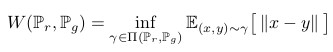
* (inf = infinum, more or less a minimum)
* which is intractable, but following the Kantorovich-Rubinstein duality it can also be calculated via
* 
* (sup = supremum, more or less a maximum)
* However, the second formula is here only valid if the network is a K-Lipschitz function (under every set of parameters).
* This can be guaranteed by simply clipping the discriminator's weights to the range `[-0.01, 0.01]`.
* Then in practice the following version of the tractable EM is used, where `w` are the parameters of the discriminator:
* 
* The full algorithm is mostly the same as for DCGAN:
* 
* Line 2 leads to training the discriminator multiple times per batch (i.e. more often than the generator).
* This is similar to the `max w in W` in the third formula (above).
* This was already part of the original GAN algorithm, but is here more actively used.
* Because of the EM distance, even a "perfect" discriminator still gives good gradient (in contrast to e.g. JS, where the discriminator should not be too far ahead). So the discriminator can be safely trained more often than the generator.
* Line 5 and 10 are derived from EM. Note that there is no more Sigmoid at the end of the discriminator!
* Line 7 is derived from the K-Lipschitz requirement (clipping of weights).
* High learning rates or using momentum-based optimizers (e.g. Adam) made the training unstable, which is why they use a small learning rate with RMSprop.
### Results
* Improved stability. The method converges to decent images with models which failed completely when using JS-divergence (like in DCGAN).
* For example, WGAN worked with generators that did not have batch normalization or only consisted of fully connected layers.
* Apparently no more mode collapse. (Mode collapse in GANs = the generator starts to generate often/always the practically same image, independent of the noise input.)
* There is a relationship between loss and image quality. Lower loss (at the generator) indicates higher image quality. Such a relationship did not exist for JS divergence.
* Example images:
* 
|
YOLO9000: Better, Faster, Stronger
Joseph Redmon and Ali Farhadi
arXiv e-Print archive - 2016 via Local arXiv
Keywords: cs.CV
First published: 2016/12/25 (9 years ago)
Abstract: We introduce YOLO9000, a state-of-the-art, real-time object detection system that can detect over 9000 object categories. First we propose various improvements to the YOLO detection method, both novel and drawn from prior work. The improved model, YOLOv2, is state-of-the-art on standard detection tasks like PASCAL VOC and COCO. At 67 FPS, YOLOv2 gets 76.8 mAP on VOC 2007. At 40 FPS, YOLOv2 gets 78.6 mAP, outperforming state-of-the-art methods like Faster RCNN with ResNet and SSD while still running significantly faster. Finally we propose a method to jointly train on object detection and classification. Using this method we train YOLO9000 simultaneously on the COCO detection dataset and the ImageNet classification dataset. Our joint training allows YOLO9000 to predict detections for object classes that don't have labelled detection data. We validate our approach on the ImageNet detection task. YOLO9000 gets 19.7 mAP on the ImageNet detection validation set despite only having detection data for 44 of the 200 classes. On the 156 classes not in COCO, YOLO9000 gets 16.0 mAP. But YOLO can detect more than just 200 classes; it predicts detections for more than 9000 different object categories. And it still runs in real-time.
more
less
Joseph Redmon and Ali Farhadi
arXiv e-Print archive - 2016 via Local arXiv
Keywords: cs.CV
First published: 2016/12/25 (9 years ago)
Abstract: We introduce YOLO9000, a state-of-the-art, real-time object detection system that can detect over 9000 object categories. First we propose various improvements to the YOLO detection method, both novel and drawn from prior work. The improved model, YOLOv2, is state-of-the-art on standard detection tasks like PASCAL VOC and COCO. At 67 FPS, YOLOv2 gets 76.8 mAP on VOC 2007. At 40 FPS, YOLOv2 gets 78.6 mAP, outperforming state-of-the-art methods like Faster RCNN with ResNet and SSD while still running significantly faster. Finally we propose a method to jointly train on object detection and classification. Using this method we train YOLO9000 simultaneously on the COCO detection dataset and the ImageNet classification dataset. Our joint training allows YOLO9000 to predict detections for object classes that don't have labelled detection data. We validate our approach on the ImageNet detection task. YOLO9000 gets 19.7 mAP on the ImageNet detection validation set despite only having detection data for 44 of the 200 classes. On the 156 classes not in COCO, YOLO9000 gets 16.0 mAP. But YOLO can detect more than just 200 classes; it predicts detections for more than 9000 different object categories. And it still runs in real-time.
|
[link]
* They suggest a new version of YOLO, a model to detect bounding boxes in images.
* Their new version is more accurate, faster and is trained to recognize up to 9000 classes.
### How
* Their base model is the previous YOLOv1, which they improve here.
* Accuracy improvements
* They add batch normalization to the network.
* Pretraining usually happens on ImageNet at 224x224, fine tuning for bounding box detection then on another dataset, say Pascal VOC 2012, at higher resolutions, e.g. 448x448 in the case of YOLOv1.
This is problematic, because the pretrained network has to learn to deal with higher resolutions and a new task at the same time.
They instead first pretrain on low resolution ImageNet examples, then on higher resolution ImegeNet examples and only then switch to bounding box detection.
That improves their accuracy by about 4 percentage points mAP.
* They switch to anchor boxes, similar to Faster R-CNN. That's largely the same as in YOLOv1. Classification is now done per tested anchor box shape, instead of per grid cell.
The regression of x/y-coordinates is now a bit smarter and uses sigmoids to only translate a box within a grid cell.
* In Faster R-CNN the anchor box shapes are manually chosen (e.g. small squared boxes, large squared boxes, thin but high boxes, ...).
Here instead they learn these shapes from data.
That is done by applying k-Means to the bounding boxes in a dataset.
They cluster them into k=5 clusters and then use the centroids as anchor box shapes.
Their accuracy this way is the same as with 9 manually chosen anchor boxes.
(Using k=9 further increases their accuracy significantly, but also increases model complexity. As they want to predict 9000 classes they stay with k=5.)
* To better predict small bounding boxes, they add a pass-through connection from a higher resolution layer to the end of the network.
* They train their network now at multiple scales. (As the network is now fully convolutional, they can easily do that.)
* Speed improvements
* They get rid of their fully connected layers. Instead the network is now fully convolutional.
* They have also removed a handful or so of their convolutional layers.
* Capability improvement (weakly supervised learning)
* They suggest a method to predict bounding boxes of the 9000 most common classes in ImageNet.
They add a few more abstract classes to that (e.g. dog for all breeds of dogs) and arrive at over 9000 classes (9418 to be precise).
* They train on ImageNet and MSCOCO.
* ImageNet only contains class labels, no bounding boxes. MSCOCO only contains general classes (e.g. "dog" instead of the specific breed).
* They train iteratively on both datasets. MSCOCO is used for detection and classification, while ImageNet is only used for classification.
For an ImageNet example of class `c`, they search among the predicted bounding boxes for the one that has highest predicted probability of being `c`
and backpropagate only the classification loss for that box.
* In order to compensate the problem of different abstraction levels on the classes (e.g. "dog" vs a specific breed), they make use of WordNet.
Based on that data they generate a hierarchy/tree of classes, e.g. one path through that tree could be: object -> animal -> canine -> dog -> hunting dog -> terrier -> yorkshire terrier.
They let the network predict paths in that hierarchy, so that the prediction "dog" for a specific dog breed is not completely wrong.
* Visualization of the hierarchy:
* 
* They predict many small softmaxes for the paths in the hierarchy, one per node:
* 
### Results
* Accuracy
* They reach about 73.4 mAP when training on Pascal VOC 2007 and 2012. That's slightly behind Faster R-CNN with VGG16 with 75.9 mAP, trained on MSCOCO+2007+2012.
* Speed
* They reach 91 fps (10ms/image) at image resolution 288x288 and 40 fps (25ms/image) at 544x544.
* Weakly supervised learning
* They test their 9000-class-detection on ImageNet's detection task, which contains bounding boxes for 200 object classes.
* They achieve 19.7 mAP for all classes and 16.0% mAP for the 156 classes which are not part of MSCOCO.
* For some classes they get 0 mAP accuracy.
* The system performs well for all kinds of animals, but struggles with not-living objects, like sunglasses.
* Example images (notice the class labels):
* 
|
You Only Look Once: Unified, Real-Time Object Detection
Redmon, Joseph and Divvala, Santosh Kumar and Girshick, Ross B. and Farhadi, Ali
Conference and Computer Vision and Pattern Recognition - 2016 via Local Bibsonomy
Keywords: dblp
Redmon, Joseph and Divvala, Santosh Kumar and Girshick, Ross B. and Farhadi, Ali
Conference and Computer Vision and Pattern Recognition - 2016 via Local Bibsonomy
Keywords: dblp
|
[link]
* They suggest a model ("YOLO") to detect bounding boxes in images.
* In comparison to Faster R-CNN, this model is faster but less accurate.
### How
* Architecture
* Input are images with a resolution of 448x448.
* Output are `S*S*(B*5 + C)` values (per image).
* `S` is the grid size (default value: 7). Each image is split up into `S*S` cells.
* `B` is the number of "tested" bounding box shapes at each cell (default value: 2).
So at each cell, the network might try one large and one small bounding box.
The network predicts additionally for each such tested bounding box `5` values.
These cover the exact position (x, y) and scale (height, width) of the bounding box as well as a confidence value.
They allow the network to fine tune the bounding box shape and reject it, e.g. if there is no object in the grid cell.
The confidence value is zero if there is no object in the grid cell and otherwise matches the IoU between predicted and true bounding box.
* `C` is the number of classes in the dataset (e.g. 20 in Pascal VOC). For each grid cell, the model decides once to which of the `C` objects the cell belongs.
* Rough overview of their outputs:
* 
* In contrast to Faster R-CNN, their model does *not* use a separate region proposal network (RPN).
* Per bounding box they actually predict the *square root* of height and width instead of the raw values.
That is supposed to result in similar errors/losses for small and big bounding boxes.
* They use a total of 24 convolutional layers and 2 fully connected layers.
* Some of these convolutional layers are 1x1-convs that halve the number of channels (followed by 3x3s that double them again).
* Overview of the architecture:
* 
* They use Leaky ReLUs (alpha=0.1) throughout the network. The last layer uses linear activations (apparently even for the class prediction...!?).
* Similarly to Faster R-CNN, they use a non maximum suppression that drops predicted bounding boxes if they are too similar to other predictions.
* Training
* They pretrain their network on ImageNet, then finetune on Pascal VOC.
* Loss
* They use sum-squared losses (apparently even for the classification, i.e. the `C` values).
* They dont propagate classification loss (for `C`) for grid cells that don't contain an object.
* For each grid grid cell they "test" `B` example shapes of bounding boxes (see above).
Among these `B` shapes, they only propagate the bounding box losses (regarding x, y, width, height, confidence) for the shape that has highest IoU with a ground truth bounding box.
* Most grid cells don't contain a bounding box. Their confidence values will all be zero, potentialle dominating the total loss.
To prevent that, the weighting of the confidence values in the loss function is reduced relative to the regression components (x, y, height, width).
### Results
* The coarse grid and B=2 setting lead to some problems. Namely, small objects are missed and bounding boxes can end up being dropped if they are too close to other bounding boxes.
* The model also has problems with unusual bounding box shapes.
* Overall their accuracy is about 10 percentage points lower than Faster R-CNN with VGG16 (63.4% vs 73.2%, measured in mAP on Pascal VOC 2007).
* They achieve 45fps (22ms/image), compared to 7fps (142ms/image) with Faster R-CNN + VGG16.
* Overview of results on Pascal VOC 2012:
* 
* They also suggest a faster variation of their model which reached 145fps (7ms/image) at a further drop of 10 percentage points mAP (to 52.7%).
* A significant part of their error seems to come from badly placed or sized bounding boxes (e.g. too wide or too much to the right).
* They mistake background less often for objects than Fast R-CNN. They test combining both models with each other and can improve Fast R-CNN's accuracy by about 2.5 percentage points mAP.
* They test their model on paintings/artwork (Picasso and People-Art datasets) and notice that it generalizes fairly well to that domain.
* Example results (notice the paintings at the top):
* 
|