"This deals with a specific prediction task, namely to predict the expression of specified target genes from a panel of about 1,000 pre-selected “landmark genes”. As the authors explain, gene expression levels are often highly correlated and it may be a cost-effective strategy in some cases to use such panels and then computationally infer the expression of other genes. Based on Pylearn2/Theano."

https://github.com/uci-cbcl/D-GEX

https://followthedata.wordpress.com/2015/12/21/list-of-deep-learning-implementations-in-biology/

The authors proposed a end-to-end way to learn how to play a game, which involves both images and text, called GuessWhat?!. They use both supervised learning as a baseline and reinforcement learning to improve their results.

**GuessWhat Rules :**

*From the paper :* "GuessWhat?! is a cooperative two-player game in which both players see the picture of a rich visual scene with several objects. One player – the oracle – is randomly assigned an object (which could be a person) in the scene. This object is not known by the other player – the questioner – whose goal is to locate the hidden object. To do so, the questioner can ask a series of yes-no questions which are answered by the oracle"

**Why do they use reinforcement learning in a dialogue context ?**

Supervised learning in a dialogue system usually brings poor results because the agent only learns to say the exact same sentences that are in the training set. Reinforcement learning seems to be a better option since it doesn't try to exactly match the sentences, but allow more flexibility as long as you get a positive reward at the end. The problem is : In a dialogue context, how can you tell that the dialogue was either "good" (positive reward) or "bad" (negative reward). In the context of the GuessWhat?! game, the reward is easy. If the guesser can find the object that the oracle was assigned to, then it gets a positive reward, otherwise it gets a negative reward.

The dataset is composed of 150k human-human dialogues.

**Models used** 

*Oracle model* : Its goal is to answer by 'yes' or 'no' to the question asked by the agent.
They are concatenating :
- LSTM encoded information of the question asked
- Information about the location of the object (coordinate of the bounding box)
- The object category

Then the vector is fed to a single hidden layer MLP
https://i.imgur.com/SjWkciI.png

*Question model* : The questionner is split in two models :
- The question generation :
    - **Input** : History of questions already asked (if questions were asked before) and the beginning of the question (if this is not the first word of the question) 
    - **Model** : LSTM with softmax
    - **Output** : The next word in the sentence
- The guesser
    - **Input** : The image + all the questions + all the answers
    - **Model** : MLP + softmax
    - **Output** : Selection of one object among the set of all objects in the image.

**Training procedure** :

Train all the components above, in a supervised way.
Once the training is done, you have a dialogue system that is good enough to play on it's own, but the question model is still pretty bad. To improve it, you can train it using REINFORCE Algorithm, the reward being positive if the question model guessed the good object, negative otherwise.

**Main Results :**

The results are given on both new objects (images have been already seen, but the objected selected had never been selected during training) and new images.
The results are in % of the human score, not in absolute accuracy (100% means human-level performance).

|                       | New objects | New images |
|-----------------------|-------------|------------|
| Baseline (Supervised) | 53.4%        | 53%         |
| Reinforce             | 63.2%        | 62%         |

We can improvement using the REINFORCE algorithm. This is mainly because supervised algorithm doesn't know when to stop asking questions and give an answer. On the other hand REINFORCE is more accurate but tends to stop too early (and giving wrong answers)

One last thing to point out regarding the database : The language learned by the agent is still pretty bad, the question are mostly "Is it ... ?" and since the oracle only answers yes/no questions, the interaction is relatively poor.

  * They suggest a new bounding box detector.
  * Their detector works without an RPN and RoI-Pooling, making it very fast (almost 60fps).
  * Their detector works at multiple scales, making it better at detecting small and large objects.
  * They achieve scores similar to Faster R-CNN.

### How
  * Architecture
    * Similar to Faster R-CNN, they use a base network (modified version of VGG16) to transform images to feature maps.
    * They do not use an RPN.
    * They predict via convolutions for each location in the feature maps:
      * (a) one confidence value per class (high confidence indicates that there is a bounding box of that class at the given location)
      * (b) x/y offsets that indicate where exactly the center of the bounding box is (e.g. a bit to the left or top of the feature map cell's center)
      * (c) height/width values that reflect the (logarithm of) the height/width of the bounding box
    * Similar to Faster R-CNN, they also use the concept of anchor boxes.
      So they generate the described values not only once per location, but several times for several anchor boxes (they use six anchor boxes).
      Each anchor box has different height/width and optionally scale.
    * Visualization of the predictions and anchor boxes:
      * ![predictions](https://github.com/aleju/papers/blob/master/neural-nets/images/SSD/predictions.jpg?raw=true "predictions")
    * They generate these predictions not only for the final feature map, but also for various feature maps in between (e.g. before pooling layers).
      This makes it easier for the network to detect small (as well as large) bounding boxes (multi-scale detection).
    * Visualization of the multi-scale architecture:
      * ![architecture](https://github.com/aleju/papers/blob/master/neural-nets/images/SSD/architecture.jpg?raw=true "architecture")
  * Training
    * Ground truth bounding boxes have to be matched with anchor boxes (at multiple scales) to determine correct outputs.
      To do this, anchor boxes and ground truth bounding boxes are matched if their jaccard overlap is 0.5 or higher.
      Any unmatched ground truth bounding box is matched to the anchor box with highest jaccard overlap.
    * Note that this means that a ground truth bounding box can be assigned to multiple anchor boxes (in Faster R-CNN it is always only one).
    * The loss function is similar to Faster R-CNN, i.e. a mixture of confidence loss (classification) and location loss (regression).
      They use softmax with crossentropy for the confidence loss and smooth L1 loss for the location.
    * Similar to Faster R-CNN, they perform hard negative mining.
      Instead of training every anchor box at every scale they only train the ones with the highest loss (per example image).
      While doing that, they also pick the anchor boxes to be trained so that 3 in 4 boxes are negative examples (and 1 in 4 positive).
    * Data Augmentation: They sample patches from images using a wide range of possible sizes and aspect ratios.
      They also horizontally flip images, perform cropping and padding and perform some photo-metric distortions.
  * Non-Maximum-Suppression (NMS)
    * Upon inference, they remove all bounding boxes that have a confidence below 0.01.
    * They then apply NMS, removing bounding boxes if there is already a similar one (measured by jaccard overlap of 0.45 or more).

### Results
  * Pascal VOC 2007
    * They achieve around 1-3 points mAP better results than Faster R-CNN.
    * ![results pascal](https://github.com/aleju/papers/blob/master/neural-nets/images/SSD/results_pascal.jpg?raw=true "results pascal")
    * Despite the multi-scale method, the model's performance is still significantly worse for small objects than for large ones.
    * Adding data augmentation significantly improved the results compared to no data augmentation (around 6 points mAP).
    * Using more than one anchor box also had noticeable effects on the results (around 2 mAP or more).
    * Using multiple feature maps to predict outputs (multi-scale architecture) significantly improves the results (around 10 mAP).
      Though adding very coarse (high-level) feature maps seems to rather hurt than help.
  * Pascal VOC 2012
    * Around 4 mAP better results than Faster R-CNN.
  * COCO
    * Between 1 and 4 mAP better results than Faster R-CNN.
  * Times
    * At a batch size of 1, SSD runs at about 46 fps at input resolution 300x300 (74.3 mAP on Pascal VOC) and 19 fps at input resolution 512x512 (76.8 mAP on Pascal VOC).
    * ![results timings](https://github.com/aleju/papers/blob/master/neural-nets/images/SSD/results_timings.jpg?raw=true "results timings")

  * They suggest a variation of Faster R-CNN.
  * Their network detects bounding boxes (e.g. of people, cars) in images *and also* segments the objects within these bounding boxes (i.e. classifies for each pixel whether it is part of the object or background).
  * The model runs roughly at the same speed as Faster R-CNN.

### How
  * The architecture and training is mostly the same as in Faster R-CNN:
    * Input is an image.
    * The *backbone* network transforms the input image into feature maps. It consists of convolutions, e.g. initialized with ResNet's weights.
    * The *RPN* (Region Proposal Network) takes the feature maps and classifies for each location whether there is a bounding box at that point (with some other stuff to regress height/width and offsets).
      This leads to a large number of bounding box candidates (region proposals) per image.
    * *RoIAlign*: Each region proposal's "area" is extracted from the feature maps and converted into a fixed-size `7x7xF` feature map (with F input filters). (See below.)
    * The *head* uses the region proposal's features to perform
      * Classification: "is the bounding box of a person/car/.../background"
      * Regression: "bounding box should have width/height/offset so and so"
      * Segmentation: "pixels so and so are part of this object's mask"
    * Rough visualization of the architecture:
      * ![Architecture](https://raw.githubusercontent.com/aleju/papers/master/neural-nets/images/Mask_R-CNN/architecture.jpg?raw=true "Architecture")
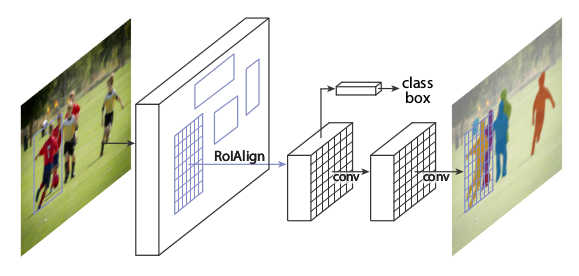
  * RoIAlign
    * This is very similar to RoIPooling in Faster R-CNN.
    * For each RoI, RoIPooling first "finds" the features in the feature maps that lie within the RoI's rectangle. Then it max-pools them to create a fixed size vector.
    * Problem: The coordinates where an RoI starts and ends may be non-integers. E.g. the top left corner might have coordinates `(x=2.5, y=4.7)`.
      RoIPooling simply rounds these values to the nearest integers (e.g. `(x=2, y=5)`).
      But that can create pooled RoIs that are significantly off, as the feature maps with which RoIPooling works have high (total) stride (e.g. 32 pixels in standard ResNets).
      So being just one cell off can easily lead to being 32 pixels off on the input image.
    * For classification, being some pixels off is usually not that bad. For masks however it can significantly worsen the results, as these have to be pixel-accurate.
    * In RoIAlign this is compensated by not rounding the coordinates and instead using bilinear interpolation to interpolate between the feature map's cells.
    * Each RoI is pooled by RoIAlign to a fixed sized feature map of size `(H, W, F)`, with H and W usually being 7 or 14. (It can also generate different sizes, e.g. `7x7xF` for classification and more accurate `14x14xF` for masks.)
    * If H and W are `7`, this leads to `49` cells within each plane of the pooled feature maps.
    * Each cell again is a rectangle -- similar to the RoIs -- and pooled with bilinear interpolation.
      More exactly, each cell is split up into four sub-cells (top left, top right, bottom right, bottom left).
      Each of these sub-cells is pooled via bilinear interpolation, leading to four values per cell.
      The final cell value is then computed using either an average or a maximum over the four sub-values.
  * Segmentation
    * They add an additional branch to the *head* that gets pooled RoI as inputs and processes them seperately from the classification and regression (no connections between the branches).
    * That branch does segmentation. It is fully convolutional, similar to many segmentation networks.
    * The result is one mask per class.
    * There is no softmax per pixel over the classes, as classification is done by a different branch.
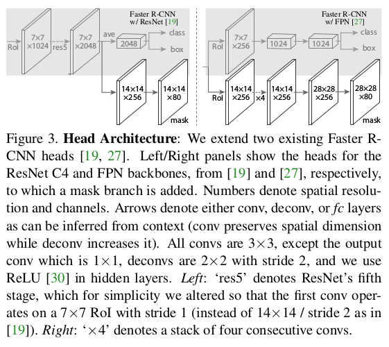
  * Base networks
    * Their *backbone* networks are either ResNet or ResNeXt (in the 50 or 102 layer variations).
    * Their *head* is either the fourth/fifth module from ResNet/ResNeXt (called *C4* (fourth) or *C5* (fifth)) or they use the second half from the FPN network (called *FPN*).
    * They denote their networks via `backbone-head`, i.e. ResNet-101-FPN means that their backbone is ResNet-101 and their head is FPN.
    * Visualization of the different heads:
      * ![Architecture heads](https://raw.githubusercontent.com/aleju/papers/master/neural-nets/images/Mask_R-CNN/head.jpg?raw=true "Architecture heads")
  * Training
    * Training happens in basically the same way as Faster R-CNN.
    * They just add an additional loss term to the total loss (`L = L_classification + L_regression + L_mask`). `L_mask` is based on binary cross-entropy.
    * For each predicted RoI, the correct mask is the intersection between that RoI's area and the correct mask.
    * They only train masks for RoIs that are positive (overlap with ground truth bounding boxes).
    * They train for 120k iterations at learning rate 0.02 and 40k at 0.002 with weight decay 0.0002 and momentum 0.9.
  * Test
    * For the *C4*-head they sample up to 300 region proposals from the RPN (those with highest confidence values). For the FPN head they sample up to 1000, as FPN is faster.
    * They sample masks only for the 100 proposals with highest confidence values.
    * Each mask is turned into a binary mask using a threshold of 0.5.

### Results
  * Instance Segmentation
    * They train and test on COCO.
    * They can outperform the best competitor by a decent margin (AP 37.1 vs 33.6 for FCIS+++ with OHEM).
    * Their model especially performs much better when there is overlap between bounding boxes.
    * Ranking of their models: ResNeXt-101-FPN > ResNet-101-FPN > ResNet-50-FPN > ResNet-101-C4 > ResNet-50-C4.
    * Using sigmoid instead of softmax (over classes) for the mask prediction significantly improves results by 5.5 to 7.1 points AP (depending on measurement method).
    * Predicting only one mask per RoI (class-agnostic) instead of C masks (where C is the number of classes) only has a small negative effect on AP (about 0.6 points).
    * Using RoIAlign instead of RoIPooling has significant positive effects on the AP of around 5 to 10 points (if a network with C5 head is chosen, which has a high stride of 32). Effects are smaller for small strides and FPN head.
    * Using fully convolutional networks for the mask branch performs better than fully connected layers (1-3 points AP).
    * Examples results on COCO vs FCIS (note the better handling of overlap):
      * ![Examples COCO](https://raw.githubusercontent.com/aleju/papers/master/neural-nets/images/Mask_R-CNN/examples_overlap.jpg?raw=true "Examples COCO")
  * Bounding-Box-Detection
    * Training additionally on masks seems to improve AP for bounding boxes by around 1 point (benefit from multi-task learning).
  * Timing
    * Around 200ms for ResNet-101-FPN. (M40 GPU)
    * Around 400ms for ResNet-101-C4.
  * Human Pose Estimation
    * The mask branch can be used to predict keypoint (landmark) locations on human bodies (i.e. locations of hands, feet etc.).
    * This is done by using one mask per keypoint, initializing it to `0` and setting the keypoint location to `1`.
    * By doing this, Mask R-CNN can predict keypoints roughly as good as the current leading models (on COCO), while running at 5fps.
  * Cityscapes
    * They test their model on the cityscapes dataset.
    * They beat previous models with significant margins. This is largely due to their better handling of overlapping instances.
    * They get their best scores using a model that was pre-trained on COCO.
    * Examples results on cityscapes:
      * ![Examples Cityscapes](https://raw.githubusercontent.com/aleju/papers/master/neural-nets/images/Mask_R-CNN/examples_cityscapes.jpg?raw=true "Examples Cityscapes")

* [Detailed Summary](https://blog.heuritech.com/2017/04/11/began-state-of-the-art-generation-of-faces-with-generative-adversarial-networks/)
* [Tensorflow implementation](https://github.com/carpedm20/BEGAN-tensorflow)

### Summary

  * They suggest a GAN algorithm that is based on an autoencoder with Wasserstein distance.
  * Their method generates highly realistic human faces.
  * Their method has a convergence measure, which reflects the quality of the generates images.
  * Their method has a diversity hyperparameter, which can be used to set the tradeoff between image diversity and image quality.

### How
  * Like other GANs, their method uses a generator G and a discriminator D.
  * Generator
    * The generator is fairly standard.
    * It gets a noise vector `z` as input and uses upsampling+convolutions to generate images.
    * It uses ELUs and no BN.
  * Discriminator
    * The discriminator is a full autoencoder (i.e. it converts input images to `8x8x3` tensors, then reconstructs them back to images).
    * It has skip-connections from the `8x8x3` layer to each upsampling layer.
    * It also uses ELUs and no BN.
  * Their method now has the following steps:
    1. Collect real images `x_real`.
    2. Generate fake images `x_fake = G(z)`.
    3. Reconstruct the real images `r_real = D(x_real)`.
    4. Reconstruct the fake images `r_fake = D(x_fake)`.
    5. Using an Lp-Norm (e.g. L1-Norm), compute the reconstruction loss of real images `d_real = Lp(x_real, r_real)`.
    6. Using an Lp-Norm (e.g. L1-Norm), compute the reconstruction loss of fake images `d_fake = Lp(x_fake, r_fake)`.
    7. The loss of D is now `L_D = d_real - d_fake`.
    8. The loss of G is now `L_G = -L_D`.
  * About the loss
    * `r_real` and `r_fake` are really losses (e.g. L1-loss or L2-loss). In the paper they use `L(...)` for that. Here they are referenced as `d_*` in order to avoid confusion.
    * The loss `L_D` is based on the Wasserstein distance, as in WGAN.
    * `L_D` assumes, that the losses `d_real` and `d_fake` are normally distributed and tries to move their mean values. Ideally, the discriminator produces very different means for real/fake images, while the generator leads to very similar means.
    * Their formulation of the Wasserstein distance does not require K-Lipschitz functions, which is why they don't have the weight clipping from WGAN.
  * Equilibrium
    * The generator and discriminator are at equilibrium, if `E[r_fake] = E[r_real]`. (That's undesirable, because it means that D can't differentiate between fake and real images, i.e. G doesn't get a proper gradient any more.)
    * Let `g = E[r_fake] / E[r_real]`, then:
      * Low `g` means that `E[r_fake]` is low and/or `E[r_real]` is high, which means that real images are not as well reconstructed as fake images. This means, that the discriminator will be more heavily trained towards reconstructing real images correctly (as that is the main source of error).
      * High `g` conversely means that real images are well reconstructed (compared to fake ones) and that the discriminator will be trained more towards fake ones.
      * `g` gives information about how much G and D should be trained each (so that none of the two overwhelms the other).
    * They introduce a hyperparameter `gamma` (from interval `[0,1]`), which reflects the target value of the balance `g`.
    * Using `gamma`, they change their losses `L_D` and `L_G` slightly:
      * `L_D = d_real - k_t d_fake`
      * `L_G = r_fake`
      * `k_t+1 = k_t + lambda_k (gamma d_real - d_fake)`.
    * `k_t` is a control term that controls how much D is supposed to focus on the fake images. It changes with every batch.
    * `k_t` is clipped to `[0,1]` and initialized at `0` (max focus on reconstructing real images).
    * `lambda_k` is like the learning rate of the control term, set to `0.001`.
    * Note that `gamma d_real - d_fake = 0 <=> gamma d_real = d_fake <=> gamma = d_fake / d_real`.
  * Convergence measure
    * They measure the convergence of their model using `M`:
    * `M = d_real + |gamma d_real - d_fake|`
    * `M` goes down, if `d_real` goes down (D becomes better at autoencoding real images).
    * `M` goes down, if the difference in reconstruction error between real and fake images goes down, i.e. if G becomes better at generating fake images.
  * Other
    * They use Adam with learning rate 0.0001. They decrease it by a factor of 2 whenever M stalls.
    * Higher initial learning rate could lead to model collapse or visual artifacs.
    * They generate images of max size 128x128.
    * They don't use more than 128 filters per conv layer.

### Results
  * NOTES:
    * Below example images are NOT from generators trained on CelebA. They used a custom dataset of celebrity images. They don't show any example images from the dataset. The generated images look like there is less background around the faces, making the task easier.
    * Few example images. Unclear how much cherry picking was involved. Though the results from the tensorflow example (see like at top) make it look like the examples are representative (aside from speckle-artifacts).
    * No LSUN Bedrooms examples. Human faces are comparatively easy to generate.
  * Example images at 128x128:
    * ![Examples](https://raw.githubusercontent.com/aleju/papers/master/neural-nets/images/BEGAN__examples.jpg?raw=true "Examples")
  * Effect of changing the target balance `gamma`:
    * ![Examples gamma](https://raw.githubusercontent.com/aleju/papers/master/neural-nets/images/BEGAN__examples_gamma.jpg?raw=true "Examples gamma")
    * High gamma leads to more diversity at lower quality.
  * Interpolations:
    * ![Interpolations](https://raw.githubusercontent.com/aleju/papers/master/neural-nets/images/BEGAN__interpolations.jpg?raw=true "Interpolations")
  * Convergence measure `M` and associated image quality during the training:
    * ![M](https://raw.githubusercontent.com/aleju/papers/master/neural-nets/images/BEGAN__convergence.jpg?raw=true "M")