* Certain activation functions, mainly sigmoid, tanh, hard-sigmoid and hard-tanh can saturate.
  * That means that their gradient is either flat 0 after threshold values (e.g. -1 and +1) or that it approaches zero for high/low values.
  * If there's no gradient, training becomes slow or stops completely.
  * That's a problem, because sigmoid, tanh, hard-sigmoid and hard-tanh are still often used in some models, like LSTMs, GRUs or Neural Turing Machines.
  * To fix the saturation problem, they add noise to the output of the activation functions.
  * The noise increases as the unit saturates.
  * Intuitively, once the unit is saturating, it will occasionally "test" an activation in the non-saturating regime to see if that output performs better.

### How
  * The basic formula is: `phi(x,z) = alpha*h(x) + (1-alpha)u(x) + d(x)std(x)epsilon`
  * Variables in that formula:
    * Non-linear part `alpha*h(x)`:
      * `alpha`: A constant hyperparameter that determines the "direction" of the noise and the slope. Values below 1.0 let the noise point away from the unsaturated regime. Values <=1.0 let it point towards the unsaturated regime (higher alpha = stronger noise).
      * `h(x)`: The original activation function.
    * Linear part `(1-alpha)u(x)`:
      * `u(x)`: First-order Taylor expansion of h(x).
        * For sigmoid: `u(x) = 0.25x + 0.5`
        * For tanh: `u(x) = x`
        * For hard-sigmoid: `u(x) = max(min(0.25x+0.5, 1), 0)`
        * For hard-tanh: `u(x) = max(min(x, 1), -1)`
    * Noise/Stochastic part `d(x)std(x)epsilon`:
      * `d(x) = -sgn(x)sgn(1-alpha)`: Changes the "direction" of the noise.
      * `std(x) = c(sigmoid(p*v(x))-0.5)^2 = c(sigmoid(p*(h(x)-u(x)))-0.5)^2`
        * `c` is a hyperparameter that controls the scale of the standard deviation of the noise.
        * `p` controls the magnitude of the noise. Due to the `sigmoid(y)-0.5` this can influence the sign. `p` is learned.
      * `epsilon`: A noise creating random variable. Usually either a Gaussian or the positive half of a Gaussian (i.e. `z` or `|z|`).
  * The hyperparameter `c` can be initialized at a high value and then gradually decreased over time. That would be comparable to simulated annealing.
  * Noise could also be applied to the input, i.e. `h(x)` becomes `h(x + noise)`.

### Results
  * They replaced sigmoid/tanh/hard-sigmoid/hard-tanh units in various experiments (without further optimizations).
  * The experiments were:
    * Learn to execute source code (LSTM?)
    * Language model from Penntreebank (2-layer LSTM)
    * Neural Machine Translation engine trained on Europarl (LSTM?)
    * Image caption generation with soft attention trained on Flickr8k (LSTM)
    * Counting unique integers in a sequence of integers (LSTM)
    * Associative recall (Neural Turing Machine)
  * Noisy activations practically always led to a small or moderate improvement in resulting accuracy/NLL/BLEU.
  * In one experiment annealed noise significantly outperformed unannealed noise, even beating careful curriculum learning. (Somehow there are not more experiments about that.)
  * The Neural Turing Machine learned far faster with noisy activations and also converged to a much better solution. 


![Influence of alphas](https://raw.githubusercontent.com/aleju/papers/master/neural-nets/images/Noisy_Activation_Functions__alphas.png?raw=true "Influence of alphas.")

*Hard-tanh with noise for various alphas. Noise increases in different ways in the saturing regimes.*


![Neural Turing Machine results](https://raw.githubusercontent.com/aleju/papers/master/neural-nets/images/Noisy_Activation_Functions__ntm.png?raw=true "Neural Turing Machine results.")

*Performance during training of a Neural Turing Machine with and without noisy activation units.*

--------------------

# Rough chapter-wise notes

* (1) Introduction
  * ReLU and Maxout activation functions have improved the capabilities of training deep networks.
  * Previously, tanh and sigmoid were used, which were only suited for shallow networks, because they saturate, which kills the gradient.
  * They suggest a different avenue: Use saturating nonlinearities, but inject noise when they start to saturate (and let the network learn how much noise is "good").
  * The noise allows to train deep networks with saturating activation functions.
  * Many current architectures (LSTMs, GRUs, Neural Turing Machines, ...) require "hard" decisions (yes/no). But they use "soft" activation functions to implement those, because hard functions lack gradient.
  * The soft activation functions can still saturate (no more gradient) and don't match the nature of the binary decision problem. So it would be good to replace them with something better.
  * They instead use hard activation functions and compensate for the lack of gradient by using noise (during training).
  * Networks with hard activation functions outperform those with soft ones.

* (2) Saturating Activation Functions
  * Activation Function = A function that maps a real value to a new real value and is differentiable almost everywhere.
  * Right saturation = The gradient of an activation function becomes 0 if the input value goes towards infinity.
  * Left saturation = The gradient of an activation function becomes 0 if the input value goes towards -infinity.
  * Saturation = A activation function saturates if it right-saturates and left-saturates.
  * Hard saturation = If there is a constant c for which for which the gradient becomes 0.
  * Soft saturation = If there is no constant, i.e. the input value must become +/- infinity.
  * Soft saturating activation functions can be converted to hard saturating ones by using a first-order Taylor expansion and then clipping the values to the required range (e.g. 0 to 1).
  * A hard activating tanh is just `f(x) = x`. With clipping to [-1, 1]: `max(min(f(x), 1), -1)`.
  * The gradient for hard activation functions is 0 above/below certain constants, which will make training significantly more challenging.
  * hard-sigmoid, sigmoid and tanh are contractive mappings, hard-tanh for some reason only when it's greater than the threshold.
  * The fixed-point for tanh is 0, for the others !=0. That can have influences on the training performance.

* (3) Annealing with Noisy Activation Functions
  * Suppose that there is an activation function like hard-sigmoid or hard-tanh with additional noise (iid, mean=0, variance=std^2).
  * If the noise's `std` is 0 then the activation function is the original, deterministic one.
  * If the noise's `std` is very high then the derivatives and gradient become high too. The noise then "drowns" signal and the optimizer just moves randomly through the parameter space.
  * Let the signal to noise ratio be `SNR = std_signal / std_noise`. So if SNR is low then noise drowns the signal and exploration is random.
  * By letting SNR grow (i.e. decreaseing `std_noise`) we switch the model to fine tuning mode (less coarse exploration).
  * That is similar to simulated annealing, where noise is also gradually decreased to focus on better and better regions of the parameter space.

* (4) Adding Noise when the Unit Saturate
  * This approach does not always add the same noise. Instead, noise is added proportinally to the saturation magnitude. More saturation, more noise.
  * That results in a clean signal in "good" regimes (non-saturation, strong gradients) and a noisy signal in "bad" regimes (saturation).
  * Basic activation function with noise: `phi(x, z) = h(x) + (mu + std(x)*z)`, where `h(x)` is the saturating activation function, `mu` is the mean of the noise, `std` is the standard deviation of the noise and `z` is a random variable.
  * Ideally the noise is unbiased so that the expectation values of `phi(x,z)` and `h(x)` are the same.
  * `std(x)` should take higher values as h(x) enters the saturating regime.
  * To calculate how "saturating" a activation function is, one can `v(x) = h(x) - u(x)`, where `u(x)` is the first-order Taylor expansion of `h(x)`.
  * Empirically they found that a good choice is `std(x) = c(sigmoid(p*v(x)) - 0.5)^2` where `c` is a hyperparameter and `p` is learned.
  * (4.1) Derivatives in the Saturated Regime
    * For values below the threshold, the gradient of the noisy activation function is identical to the normal activation function.
    * For values above the threshold, the gradient of the noisy activation function is `phi'(x,z) = std'(x)*z`. (Assuming that z is unbiased so that mu=0.)
  * (4.2) Pushing Activations towards the Linear Regime
    * In saturated regimes, one would like to have more of the noise point towards the unsaturated regimes than away from them (i.e. let the model try often whether the unsaturated regimes might be better).
    * To achieve this they use the formula `phi(x,z) = alpha*h(x) + (1-alpha)u(x) + d(x)std(x)epsilon`
      * `alpha`: A constant hyperparameter that determines the "direction" of the noise and the slope. Values below 1.0 let the noise point away from the unsaturated regime. Values <=1.0 let it point towards the unsaturated regime (higher alpha = stronger noise).
      * `h(x)`: The original activation function.
      * `u(x)`: First-order Taylor expansion of h(x).
      * `d(x) = -sgn(x)sgn(1-alpha)`: Changes the "direction" of the noise.
      * `std(x) = c(sigmoid(p*v(x))-0.5)^2 = c(sigmoid(p*(h(x)-u(x)))-0.5)^2` with `c` being a hyperparameter and `p` learned.
      * `epsilon`: Either `z` or `|z|`. If `z` is a Gaussian, then `|z|` is called "half-normal" while just `z` is called "normal". Half-normal lets the noise only point towards one "direction" (towards the unsaturated regime or away from it), while normal noise lets it point in both directions (with the slope being influenced by `alpha`).
    * The formula can be split into three parts:
      * `alpha*h(x)`: Nonlinear part.
      * `(1-alpha)u(x)`: Linear part.
      * `d(x)std(x)epsilon`: Stochastic part.
    * Each of these parts resembles a path along which gradient can flow through the network.
    * During test time the activation function is made deterministic by using its expectation value: `E[phi(x,z)] = alpha*h(x) + (1-alpha)u(x) + d(x)std(x)E[epsilon]`.
    * If `z` is half-normal then `E[epsilon] = sqrt(2/pi)`. If `z` is normal then `E[epsilon] = 0`.

* (5) Adding Noise to Input of the Function
  * Noise can also be added to the input of an activation function, i.e. `h(x)` becomes `h(x + noise)`.
  * The noise can either always be applied or only once the input passes a threshold.

* (6) Experimental Results
  * They applied noise only during training.
  * They used existing setups and just changed the activation functions to noisy ones. No further optimizations.
  * `p` was initialized uniformly to [-1,1].
  * Basic experiment settings:
    * NAN: Normal noise applied to the outputs.
    * NAH: Half-normal noise, i.e. `|z|`, i.e. noise is "directed" towards the unsaturated or satured regime.
    * NANI: Normal noise applied to the *input*, i.e. `h(x+noise)`.
    * NANIL: Normal noise applied to the input with learned variance.
    * NANIS: Normal noise applied to the input, but only if the unit saturates (i.e. above/below thresholds).
  * (6.1) Exploratory analysis
    * A very simple MNIST network performed slightly better with noisy activations than without. But comparison was only to tanh and hard-tanh, not ReLU or similar.
    * In an experiment with a simple GRU, NANI (noisy input) and NAN (noisy output) performed practically identical. NANIS (noisy input, only when saturated) performed significantly worse.
  * (6.2) Learning to Execute
    * Problem setting: Predict the output of some lines of code.
    * They replaced sigmoids and tanhs with their noisy counterparts (NAH, i.e. half-normal noise on output). The model learned faster.
  * (6.3) Penntreebank Experiments
    * They trained a standard 2-layer LSTM language model on Penntreebank.
    * Their model used noisy activations, as opposed to the usually non-noisy ones.
    * They could improve upon the previously best value. Normal noise and half-normal noise performed roughly the same.
  * (6.4) Neural Machine Translation Experiments
    * They replaced all sigmoids and tanh units in the Neural Attention Model with noisy ones. Then they trained on the Europarl corpus.
    * They improved upon the previously best score.
  * (6.5) Image Caption Generation Experiments
    * They train a network with soft attention to generate captions for the Flickr8k dataset.
    * Using noisy activation units improved the result over normal sigmoids and tanhs.
  * (6.6) Experiments with Continuation
    * They build an LSTM and train it to predict how many unique integers there are in a sequence of random integers.
    * Instead of using a constant value for hyperparameter `c` of the noisy activations (scale of the standard deviation of the noise), they start at `c=30` and anneal down to `c=0.5`.
    * Annealed noise performed significantly better then unannealed noise.
    * Noise applied to the output (NAN) significantly beat noise applied to the input (NANIL).
    * In a second experiment they trained a Neural Turing Machine on the associative recall task.
    * Again they used annealed noise.
    * The NTM with annealed noise learned by far faster than the one without annealed noise and converged to a perfect solution.

https://www.youtube.com/watch?v=vQk_Sfl7kSc&feature=youtu.be

  * The paper describes a method to transfer the style (e.g. choice of colors, structure of brush strokes) of an image to a whole video.
  * The method is designed so that the transfered style is consistent over many frames.
  * Examples for such consistency:
    * No flickering of style between frames. So the next frame has always roughly the same style in the same locations.
    * No artefacts at the boundaries of objects, even if they are moving.
    * If an area gets occluded and then unoccluded a few frames later, the style of that area is still the same as before the occlusion.

### How
  * Assume that we have a frame to stylize $x$ and an image from which to extract the style $a$.
  * The basic process is the same as in the original Artistic Style Transfer paper, they just add a bit on top of that.
  * They start with a gaussian noise image $x'$ and change it gradually so that a loss function gets minimized.
  * The loss function has the following components:
    * Content loss *(old, same as in the Artistic Style Transfer paper)*
      * This loss makes sure that the content in the generated/stylized image still matches the content of the original image.
      * $x$ and $x'$ are fed forward through a pretrained network (VGG in their case).
      * Then the generated representations of the intermediate layers of the network are extracted/read.
      * One or more layers are picked and the difference between those layers for $x$ and $x'$ is measured via a MSE.
      * E.g. if we used only the representations of the layer conv5 then we would get something like `(conv5(x) - conv5(x'))^2` per example. (Where conv5() also executes all previous layers.)
    * Style loss *(old)*
      * This loss makes sure that the style of the generated/stylized image matches the style source $a$.
      * $x'$ and $a$ are fed forward through a pretrained network (VGG in their case).
      * Then the generated representations of the intermediate layers of the network are extracted/read.
      * One or more layers are picked and the Gram Matrices of those layers are calculated.
      * Then the difference between those matrices is measured via a MSE.
    * Temporal loss *(new)*
      * This loss enforces consistency in style between a pair of frames.
      * The main sources of inconsistency are boundaries of moving objects and areas that get unonccluded.
      * They use the optical flow to detect motion.
        * Applying an optical flow method to two frames $(i, i+1)$ returns per pixel the movement of that pixel, i.e. if the pixel at $(x=1, y=2)$ moved to $(x=2, y=4)$ the optical flow at that pixel would be $(u=1, v=2)$.
        * The optical flow can be split into the forward flow (here `fw`) and the backward flow (here `bw`). The forward flow is the flow from frame i to i+1 (as described in the previous point). The backward flow is the flow from frame $i+1$ to $i$ (reverse direction in time).
      * Boundaries
        * At boundaries of objects the derivative of the flow is high, i.e. the flow "suddenly" changes significantly from one pixel to the other.
        * So to detect boundaries they use (per pixel) roughly the equation `gradient(u)^2 + gradient(v)^2 > length((u,v))`.
      * Occlusions and disocclusions
        * If a pixel does not get occluded/disoccluded between frames, the optical flow method should be able to correctly estimate the motion of that pixel between the frames. The forward and backward flows then should be roughly equal, just in opposing directions.
        * If a pixel does get occluded/disoccluded between frames, it will not be visible in one the two frames and therefore the optical flow method cannot reliably estimate the motion for that pixel. It is then expected that the forward and backward flow are unequal.
        * To measure that effect they roughly use (per pixel) a formula matching `length(fw + bw)^2 > length(fw)^2 + length(bw)^2`.
      * Mask $c$
        * They create a mask $c$ with the size of the frame.
        * For every pixel they estimate whether the boundary-equation *or* the disocclusion-equation is true.
        * If either of them is true, they add a 0 to the mask, otherwise a 1. So the mask is 1 wherever there is *no* disocclusion or motion boundary.
      * Combination
        * The final temporal loss is the mean (over all pixels) of $c*(x-w)^2$.
          * $x$ is the frame to stylize.
          * $w$ is the previous *stylized* frame (frame i-1), warped according to the optical flow between frame i-1 and i.
          * `c` is the mask value at the pixel.
        * By using the difference `x-w` they ensure that the difference in styles between two frames is low.
        * By adding `c` they ensure the style-consistency only at pixels that probably should have a consistent style.
    * Long-term loss *(new)*
      * This loss enforces consistency in style between pairs of frames that are longer apart from each other.
      * It is a simple extension of the temporal (short-term) loss.
      * The temporal loss was computed for frames (i-1, i). The long-term loss is the sum of the temporal losses for the frame pairs {(i-4,i), (i-2,i), (i-1,i)}.
      * The $c$ mask is recomputed for every pair and 1 if there are no boundaries/disocclusions detected, but only if there is not a 1 for the same pixel in a later mask. The additional condition is intended to associate pixels with their closest neighbours in time to minimize possible errors.
      * Note that the long-term loss can completely replace the temporal loss as the latter one is contained in the former one.
  * Multi-pass approach *(new)*
    * They had problems with contrast around the boundaries of the frames.
    * To combat that, they use a multi-pass method in which they seem to calculate the optical flow in multiple forward and backward passes? (Not very clear here what they do and why it would help.)
  * Initialization with previous frame *(new)*
    * Instead of starting at a gaussian noise image every time, they instead use the previous stylized frame.
    * That immediately leads to more similarity between the frames.

  * They present a model which adds color to grayscale images (e.g. to old black and white images).
  * It works best with 224x224 images, but can handle other sizes too.

### How
  * Their model has three feature extraction components:
    * Low level features:
      * Receives 1xHxW images and outputs 512xH/8xW/8 matrices.
      * Uses 6 convolutional layers (3x3, strided, ReLU) for that.
    * Global features:
      * Receives the low level features and converts them to 256 dimensional vectors.
      * Uses 4 convolutional layers (3x3, strided, ReLU) and 3 fully connected layers (1024 -> 512 -> 256; ReLU) for that.
    * Mid-level features:
      * Receives the low level features and converts them to 256xH/8xW/8 matrices.
      * Uses 2 convolutional layers (3x3, ReLU) for that.
  * The global and mid-level features are then merged with a Fusion Layer.
    * The Fusion Layer is basically an extended convolutional layer.
    * It takes the mid-level features (256xH/8xW/8) and the global features (256) as input and outputs a matrix of shape 256xH/8xW/8.
    * It mostly operates like a normal convolutional layer on the mid-level features. However, its weight matrix is extended to also include weights for the global features (which will be added at every pixel).
    * So they use something like `fusion at pixel u,v = sigmoid(bias + weights * [global features, mid-level features at pixel u,v])` - and that with 256 different weight matrices and biases for 256 filters.
  * After the Fusion Layer they use another network to create the coloring:
    * This network receives 256xH/8xW/8 matrices (merge of global and mid-level features) and generates 2xHxW outputs (color in L\*a\*b\* color space).
    * It uses a few convolutional layers combined with layers that do nearest neighbour upsampling.
  * The loss for the colorization network is a MSE based on the true coloring.
  * They train the global feature extraction also on the true class labels of the used images.
  * Their model can handle any sized image. If the image doesn't have a size of 224x224, it must be resized to 224x224 for the gobal feature extraction. The mid-level feature extraction only uses convolutions, therefore it can work with any image size. 

### Results
  * The training set that they use is the "Places scene dataset".
  * After cleanup the dataset contains 2.3M training images (205 different classes) and 19k validation images.
  * Users rate images colored by their method in 92.6% of all cases as real-looking (ground truth: 97.2%).
  * If they exclude global features from their method, they only achieve 70% real-looking images.
  * They can also extract the global features from image A and then use them on image B. That transfers the style from A to B. But it only works well on semantically similar images.

![Architecture](https://raw.githubusercontent.com/aleju/papers/master/neural-nets/images/Let_there_be_Color__architecture.png?raw=true "Architecture")

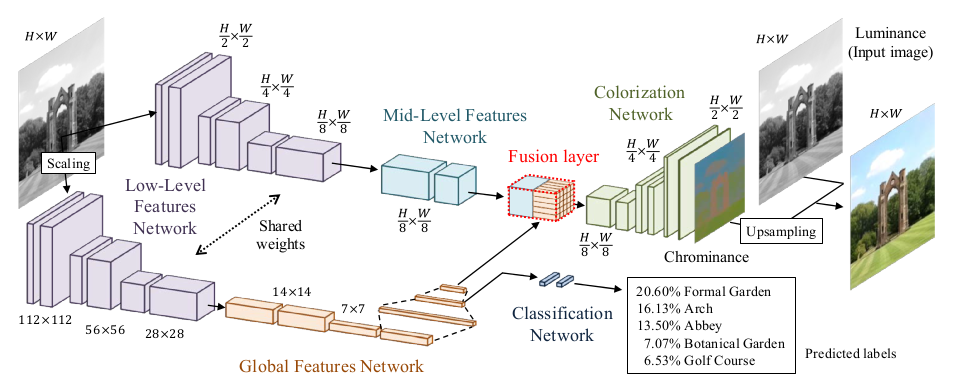
*Architecture of their model.*


![Old images](https://raw.githubusercontent.com/aleju/papers/master/neural-nets/images/Let_there_be_Color__old_images.png?raw=true "Old images")

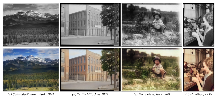
*Their model applied to old images.*

--------------------

# Rough chapter-wise notes

* (1) Introduction
  * They use a CNN to color images.
  * Their network extracts global priors and local features from grayscale images.
  * Global priors:
    * Extracted from the whole image (e.g. time of day, indoor or outdoors, ...).
    * They use class labels of images to train those. (Not needed during test.)
  * Local features: Extracted from small patches (e.g. texture).
  * They don't generate a full RGB image, instead they generate the chrominance map using the CIE L\*a\*b\* colorspace.
  * Components of the model:
    * Low level features network: Generated first.
    * Mid level features network: Generated based on the low level features.
    * Global features network: Generated based on the low level features.
    * Colorization network: Receives mid level and global features, which were merged in a fusion layer.
  * Their network can process images of arbitrary size.
  * Global features can be generated based on another image to change the style of colorization, e.g. to change the seasonal colors from spring to summer.

* (3) Joint Global and Local Model
  * <repetition of parts of the introduction>
  * They mostly use ReLUs.
  * (3.1) Deep Networks
    * <standard neural net introduction>
  * (3.2) Fusing Global and Local Features for Colorization
    * Global features are used as priors for local features.
    * (3.2.1) Shared Low-Level Features
      * The low level features are which's (low level) features are fed into the networks of both the global and the medium level features extractors.
      * They generate them from the input image using a ConvNet with 6 layers (3x3, 1x1 padding, strided/no pooling, ends in 512xH/8xW/8).
    * (3.2.2) Global Image Features
      * They process the low level features via another network into global features.
      * That network has 4 conv-layers (3x3, 2 strided layers, all 512 filters), followed by 3 fully connected layers (1024, 512, 256).
      * Input size (of low level features) is expected to be 224x224.
    * (3.2.3) Mid-Level Features
      * Takes the low level features (512xH/8xW/8) and uses 2 conv layers (3x3) to transform them to 256xH/8xW/8.
    * (3.2.4) Fusing Global and Local Features
      * The Fusion Layer is basically an extended convolutional layer.
      * It takes the mid-level features (256xH/8xW/8) and the global features (256) as input and outputs a matrix of shape 256xH/8xW/8.
      * It mostly operates like a normal convolutional layer on the mid-level features. However, its weight matrix is extended to also include weights for the global features (which will be added at every pixel).
      * So they use something like `fusion at pixel u,v = sigmoid(bias + weights * [global features, mid-level features at pixel u,v])` - and that with 256 different weight matrices and biases for 256 filters.
    * (3.2.5) Colorization Network
      * The colorization network receives the 256xH/8xW/8 matrix from the fusion layer and transforms it to the 2xHxW chrominance map.
      * It basically uses two upsampling blocks, each starting with a nearest neighbour upsampling layer, followed by 2 3x3 convs.
      * The last layer uses a sigmoid activation.
      * The network ends in a MSE.
  * (3.3) Colorization with Classification
    * To make training more effective, they train parts of the global features network via image class labels.
    * I.e. they take the output of the 2nd fully connected layer (at the end of the global network), add one small hidden layer after it, followed by a sigmoid output layer (size equals number of class labels).
    * They train that with cross entropy. So their global loss becomes something like `L = MSE(color accuracy) + alpha*CrossEntropy(class labels accuracy)`.
  * (3.4) Optimization and Learning
    * Low level feature extraction uses only convs, so they can be extracted from any image size.
    * Global feature extraction uses fc layers, so they can only be extracted from 224x224 images.
    * If an image has a size unequal to 224x224, it must be (1) resized to 224x224, fed through low level feature extraction, then fed through the global feature extraction and (2) separately (without resize) fed through the low level feature extraction and then fed through the mid-level feature extraction.
    * However, they only trained on 224x224 images (for efficiency).
    * Augmentation: 224x224 crops from 256x256 images; random horizontal flips.
    * They use Adadelta, because they don't want to set learning rates. (Why not adagrad/adam/...?)

* (4) Experimental Results and Discussion
  * They set the alpha in their loss to `1/300`.
  * They use the "Places scene dataset". They filter images with low color variance (including grayscale images). They end up with 2.3M training images and 19k validation images. They have 205 classes.
  * Batch size: 128.
  * They train for about 11 epochs.
  * (4.1) Colorization results
    * Good looking colorization results on the Places scene dataset.
  * (4.2) Comparison with State of the Art
    * Their method succeeds where other methods fail.
    * Their method can handle very different kinds of images.
  * (4.3) User study
    * When rated by users, 92.6% think that their coloring is real (ground truth: 97.2%).
    * Note: Users were told to only look briefly at the images.
  * (4.4) Importance of Global Features
    * Their model *without* global features only achieves 70% user rating.
    * There are too many ambiguities on the local level.
  * (4.5) Style Transfer through Global Features
    * They can perform style transfer by extracting the global features of image B and using them for image A.
  * (4.6) Colorizing the past
    * Their model performs well on old images despite the artifacts commonly found on those.
  * (4.7) Classification Results
    * Their method achieves nearly as high classification accuracy as VGG (see classification loss for global features).
  * (4.8) Comparison of Color Spaces
    * L\*a\*b\* color space performs slightly better than RGB and YUV, so they picked that color space.
  * (4.9) Computation Time
    * One image is usually processed within seconds.
    * CPU takes roughly 5x longer.
  * (4.10) Limitations and Discussion
    * Their approach is data driven, i.e. can only deal well with types of images that appeared in the dataset.
    * Style transfer works only really well for semantically similar images.
    * Style transfer cannot necessarily transfer specific colors, because the whole model only sees the grayscale version of the image.
    * Their model tends to strongly prefer the most common color for objects (e.g. grass always green).

  * They present a hierarchical method for reinforcement learning.
  * The method combines "long"-term goals with short-term action choices.

### How
  * They have two components:
    * Meta-Controller:
      * Responsible for the "long"-term goals.
      * Is trained to pick goals (based on the current state) that maximize (extrinsic) rewards, just like you would usually optimize to maximize rewards by picking good actions.
      * The Meta-Controller only picks goals when the Controller terminates or achieved the goal.
    * Controller:
      * Receives the current state and the current goal.
      * Has to pick a reward maximizing action based on those, just as the agent would usually do (only the goal is added here).
      * The reward is intrinsic. It comes from the Critic. The Critic gives reward whenever the current goal is reached.
  * For Montezuma's Revenge:
    * A goal is to reach a specific object.
    * The goal is encoded via a bitmask (as big as the game screen). The mask contains 1s wherever the object is.
    * They hand-extract the location of a few specific objects.
    * So basically:
      * The Meta-Controller picks the next object to reach via a Q-value function.
      * It receives extrinsic reward when objects have been reached in a specific sequence.
      * The Controller picks actions that lead to reaching the object based on a Q-value function. It iterates action-choosing until it terminates or reached the goal-object.
      * The Critic awards intrinsic reward to the Controller whenever the goal-object was reached.
    * They use CNNs for the Meta-Controller and the Controller, similar in architecture to the Atari-DQN paper (shallow CNNs).
    * They use two replay memories, one for the Meta-Controller (size 40k) and one for the Controller (size 1M).
    * Both follow an epsilon-greedy policy (for picking goals/actions). Epsilon starts at 1.0 and is annealed down to 0.1.
    * They use a discount factor / gamma of 0.9.
    * They train with SGD. 

### Results
  * Learns to play Montezuma's Revenge.
  * Learns to act well in a more abstract MDP with delayed rewards and where simple Q-learning failed.

--------------------

# Rough chapter-wise notes


* (1) Introduction
  * Basic problem: Learn goal directed behaviour from sparse feedbacks.
  * Challenges:
    * Explore state space efficiently
    * Create multiple levels of spatio-temporal abstractions
  * Their method: Combines deep reinforcement learning with hierarchical value functions.
  * Their agent is motivated to solve specific intrinsic goals.
  * Goals are defined in the space of entities and relations, which constraints the search space.
  * They define their value function as V(s, g) where s is the state and g is a goal.
  * First, their agent learns to solve intrinsically generated goals. Then it learns to chain these goals together.
  * Their model has two hiearchy levels:
    * Meta-Controller: Selects the current goal based on the current state.
    * Controller: Takes state s and goal g, then selects a good action based on s and g. The controller operates until g is achieved, then the meta-controller picks the next goal.
  * Meta-Controller gets extrinsic rewards, controller gets intrinsic rewards.
  * They use SGD to optimize the whole system (with respect to reward maximization).

* (3) Model
  * Basic setting: Action a out of all actions A, state s out of S, transition function T(s,a)->s', reward by state F(s)->R.
  * epsilon-greedy is good for local exploration, but it's not good at exploring very different areas of the state space.
  * They use intrinsically motivated goals to better explore the state space.
  * Sequences of goals are arranged to maximize the received extrinsic reward.
  * The agent learns one policy per goal.
  * Meta-Controller: Receives current state, chooses goal.
  * Controller: Receives current state and current goal, chooses action. Keeps choosing actions until goal is achieved or a terminal state is reached. Has the optimization target of maximizing cumulative reward.
  * Critic: Checks if current goal is achieved and if so provides intrinsic reward.
  * They use deep Q learning to train their model.
  * There are two Q-value functions. One for the controller and one for the meta-controller.
  * Both formulas are extended by the last chosen goal g.
  * The Q-value function of the meta-controller does not depend on the chosen action.
  * The Q-value function of the controller receives only intrinsic direct reward, not extrinsic direct reward.
  * Both Q-value functions are reprsented with DQNs.
  * Both are optimized to minimize MSE losses.
  * They use separate replay memories for the controller and meta-controller.
  * A memory is added for the meta-controller whenever the controller terminates.
  * Each new goal is picked by the meta-controller epsilon-greedy (based on the current state).
  * The controller picks actions epsilon-greedy (based on the current state and goal).
  * Both epsilons are annealed down.

* (4) Experiments
  * (4.1) Discrete MDP with delayed rewards
    * Basic MDP setting, following roughly: Several states (s1 to s6) organized in a chain. The agent can move left or right. It gets high reward if it moves to state s6 and then back to s1, otherwise it gets small reward per reached state.
    * They use their hierarchical method, but without neural nets.
    * Baseline is Q-learning without a hierarchy/intrinsic rewards.
    * Their method performs significantly better than the baseline.
  * (4.2) ATARI game with delayed rewards
    * They play Montezuma's Revenge with their method, because that game has very delayed rewards.
    * They use CNNs for the controller and meta-controller (architecture similar to the Atari-DQN paper).
    * The critic reacts to (entity1, relation, entity2) relationships. The entities are just objects visible in the game. The relation is (apparently ?) always "reached", i.e. whether object1 arrived at object2.
    * They extract the objects manually, i.e. assume the existance of a perfect unsupervised object detector.
    * They encode the goals apparently not as vectors, but instead just use a bitmask (game screen heightand width), which has 1s at the pixels that show the object.
    * Replay memory sizes: 1M for controller, 50k for meta-controller.
    * gamma=0.99
    * They first only train the controller (i.e. meta-controller completely random) and only then train both jointly.
    * Their method successfully learns to perform actions which lead to rewards with long delays.
    * It starts with easier goals and then learns harder goals.

  * They describe a model for human pose estimation, i.e. one that finds the joints ("skeleton") of a person in an image.
  * They argue that part of their model resembles a Markov Random Field (but in reality its implemented as just one big neural network).

### How
  * They have two components in their network:
    * Part-Detector:
      * Finds candidate locations for human joints in an image.
      * Pretty standard ConvNet. A few convolutional layers with pooling and ReLUs.
      * They use two branches: A fine and a coarse one. Both branches have practically the same architecture (convolutions, pooling etc.). The coarse one however receives the image downscaled by a factor of 2 (half width/height) and upscales it by a factor of 2 at the end of the branch.
      * At the end they merge the results of both branches with more convolutions.
      * The output of this model are 4 heatmaps (one per joint? unclear), each having lower resolution than the original image.
    * Spatial-Model:
      * Takes the results of the part detector and tries to remove all detections that were false positives.
      * They derive their architecture from a fully connected Markov Random Field which would be solved with one step of belief propagation.
      * They use large convolutions (128x128) to resemble the "fully connected" part.
      * They initialize the weights of the convolutions with joint positions gathered from the training set.
      * The convolutions are followed by log(), element-wise additions and exp() to resemble an energy function.
      * The end result are the input heatmaps, but cleaned up.

### Results
  * Beats all previous models (with and without spatial model).
  * Accuracy seems to be around 90% (with enough (16px) tolerance in pixel distance from ground truth).
  * Adding the spatial model adds a few percentage points of accuracy.
  * Using two branches instead of one (in the part detector) adds a bit of accuracy. Adding a third branch adds a tiny bit more.

![Results](https://raw.githubusercontent.com/aleju/papers/master/neural-nets/images/Joint_Training_of_a_ConvNet_and_a_PGM_for_HPE__results.png?raw=true "Results")

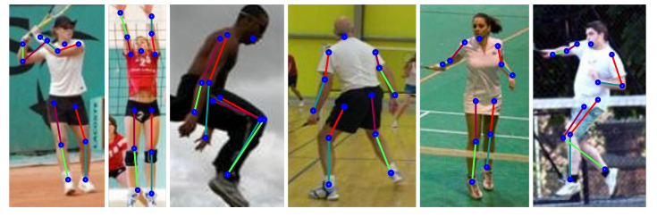
*Example results.*

![Part Detector](https://raw.githubusercontent.com/aleju/papers/master/neural-nets/images/Joint_Training_of_a_ConvNet_and_a_PGM_for_HPE__part_detector.png?raw=true "Part Detector")

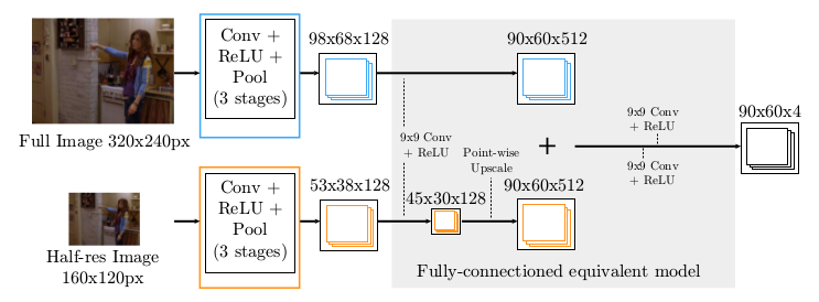
*Part Detector network.*

![Spatial Model](https://raw.githubusercontent.com/aleju/papers/master/neural-nets/images/Joint_Training_of_a_ConvNet_and_a_PGM_for_HPE__spatial_model.png?raw=true "Spatial Model")

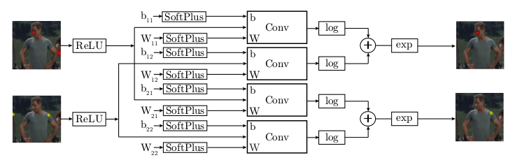
*Spatial Model (apparently only for two input heatmaps).*

-------------------------

# Rough chapter-wise notes

* (1) Introduction
  * Human Pose Estimation (HPE) from RGB images is difficult due to the high dimensionality of the input.
  * Approaches:
    * Deformable-part models: Traditionally based on hand-crafted features.
    * Deep-learning based disciminative models: Recently outperformed other models. However, it is hard to incorporate priors (e.g. possible joint- inter-connectivity) into the model.
  * They combine:
    * A part-detector (ConvNet, utilizes multi-resolution feature representation with overlapping receptive fields)
    * Part-based Spatial-Model (approximates loopy belief propagation)
  * They backpropagate through the spatial model and then the part-detector.

* (3) Model
  * (3.1) Convolutional Network Part-Detector
    * This model locates possible positions of human key joints in the image ("part detector").
    * Input: RGB image.
    * Output: 4 heatmaps, one per key joint (per pixel: likelihood).
    * They use a fully convolutional network.
    * They argue that applying convolutions to every pixel is similar to moving a sliding window over the image.
    * They use two receptive field sizes for their "sliding window": A large but coarse/blurry one, a small but fine one.
    * To implement that, they use two branches. Both branches are mostly identical (convolutions, poolings, ReLU). They simply feed a downscaled (half width/height) version of the input image into the coarser branch. At the end they upscale the coarser branch once and then merge both branches. 
    * After the merge they apply 9x9 convolutions and then 1x1 convolutions to get it down to 4xHxW (H=60, W=90 where expected input was H=320, W=240).
  * (3.2) Higher-level Spatial-Model
    * This model takes the detected joint positions (heatmaps) and tries to remove those that are probably false positives.
    * It is a ConvNet, which tries to emulate (1) a Markov Random Field and (2) solving that MRF approximately via one step of belief propagation.
    * The raw MRF formula would be something like `<likelihood of joint A per px> = normalize( <product over joint v from joints V> <probability of joint A per px given a> * <probability of joint v at px?> + someBiasTerm)`.
    * They treat the probabilities as energies and remove from the formula the partition function (`normalize`) for various reasons (e.g. because they are only interested in the maximum value anyways).
    * They use exp() in combination with log() to replace the product with a sum.
    * They apply SoftPlus and ReLU so that the energies are always positive (and therefore play well with log).
    * Apparently `<probability of joint v at px?>` are the input heatmaps of the part detector.
    * Apparently `<probability of joint A per px given a>` is implemented as the weights of a convolution.
    * Apparently `someBiasTerm` is implemented as the bias of a convolution.
    * The convolutions that they use are large (128x128) to emulate a fully connected graph.
    * They initialize the convolution weights based on histograms gathered from the dataset (empirical distribution of joint displacements).
  * (3.3) Unified Models
    * They combine the part-based model and the spatial model to a single one.
    * They first train only the part-based model, then only the spatial model, then both.

* (4) Results
  * Used datasets: FLIC (4k training images, 1k test, mostly front-facing and standing poses), FLIC-plus (17k, 1k ?), extended-LSP (10k, 1k).
  * FLIC contains images showing multiple persons with only one being annotated. So for FLIC they add a heatmap of the annotated body torso to the input (i.e. the part-detector does not have to search for the person any more).
  * The evaluation metric roughly measures, how often predicted joint positions are within a certain radius of the true joint positions.
  * Their model performs significantly better than competing models (on both FLIC and LSP).
  * Accuracy seems to be at around 80%-95% per joint (when choosing high enough evaluation tolerance, i.e. 10px+).
  * Adding the spatial model to the part detector increases the accuracy by around 10-15 percentage points.
  * Training the part detector and the spatial model jointly adds ~3 percentage points accuracy over training them separately.
  * Adding the second filter bank (coarser branch in the part detector) adds around 5 percentage points accuracy. Adding a third filter bank adds a tiny bit more accuracy.