* Stochastic Depth (SD) is a method for residual networks, which randomly removes/deactivates residual blocks during training.
  * As such, it is similar to dropout.
  * While dropout removes neurons, SD removes blocks (roughly the layers of a residual network).
  * One can argue that dropout randomly changes the width of layers, while SD randomly changes the depth of the network.
  * One can argue that using dropout is similar to training an ensemble of networks with different layer widths, while using SD is similar to training an ensemble of networks with different depths.
  * Using SD has the following advantages:
    * It decreases the effects of vanishing gradients, because on average the network is shallower during training (per batch), thereby increasing the gradient that reaches the early blocks.
    * It increases training speed, because on average less convolutions have to be applied (due to blocks being removed).
    * It has a regularizing effect, because blocks cannot easily co-adapt any more. (Similar to dropout avoiding co-adaption of neurons.)
    * If using an increasing removal probability for later blocks: It spends more training time on the early (and thus most important) blocks than on the later blocks.

### How
  * Normal formula for a residual block (test and train):
    * `output = ReLU(f(input) + identity(input))`
    * `f(x)` are usually one or two convolutions.
  * Formula with SD (during training):
    * `output = ReLU(b * f(input) + identity(input))`
    * `b` is either exactly `1` (block survived, i.e. is not removed) or exactly `0` (block was removed).
    * `b` is sampled from a bernoulli random variable that has the hyperparameter `p`.
    * `p` is the survival probability of a block (i.e. chance to *not* be removed). (Note that this is the opposite of dropout, where higher values lead to more removal.)
  * Formula with SD (during test):
    * `output = ReLU(p * f(input) + input)`
    * `p` is the average probability with which this residual block survives during training, i.e. the hyperparameter for the bernoulli variable.
    * The test formula has to be changed, because the network will adapt during training to blocks being missing. Activating them all at the same time can lead to overly strong signals. This is similar to dropout, where weights also have to be changed during test.
  * There are two simple schemas to set `p` per layer:
    * Uniform schema: Every block gets the same `p` hyperparameter, i.e. the last block has the same chance of survival as the first block.
    * Linear decay schema: Survival probability is higher for early layers and decreases towards the end.
      * The formula is `p = 1 - (l/L)(1-q)`.
      * `l`: Number of the block for which to set `p`.
      * `L`: Total number of blocks.
      * `q`: Desired survival probability of the last block (0.5 is a good value).
  * For linear decay with `q=0.5` and `L` blocks, on average `(3/4)L` blocks will be trained per minibatch.
  * For linear decay with `q=0.5` the average speedup will be about `1/4` (25%). If using `q=0.2` the speedup will be ~40%.

### Results
  * 152 layer networks with SD outperform identical networks without SD on CIFAR-10, CIFAR-100 and SVHN.
  * The improvement in test error is quite significant.
  * SD seems to have a regularizing effect. Networks with SD are not overfitting where networks without SD already are.
  * Even networks with >1000 layers are well trainable with SD.
  * The gradients that reach the early blocks of the networks are consistently significantly higher with SD than without SD (i.e. less vanishing gradient).
  * The linear decay schema consistently outperforms the uniform schema (in test error). The best value seems to be `q=0.5`, though values between 0.4 and 0.8 all seem to be good. For the uniform schema only 0.8 seems to be good.

![SVHN 152 layers](https://raw.githubusercontent.com/aleju/papers/master/neural-nets/images/Deep_Networks_with_Stochastic_Depth__svhn.png?raw=true "SVHN 152 layers")

*Performance on SVHN with 152 layer networks with SD (blue, bottom) and without SD (red, top).*


![CIFAR-10 1202 layers](https://raw.githubusercontent.com/aleju/papers/master/neural-nets/images/Deep_Networks_with_Stochastic_Depth__svhn1202.png?raw=true "CIFAR-10 1202 layers")

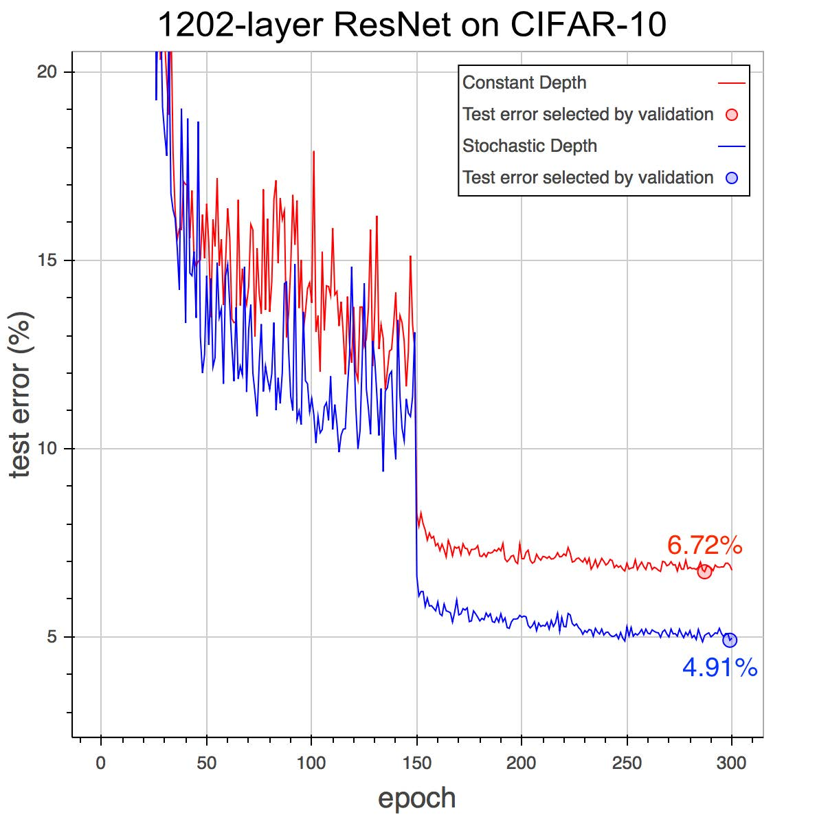
*Performance on CIFAR-10 with 1202 layer networks with SD (blue, bottom) and without SD (red, top).*


![Optimal choice of p_L](https://raw.githubusercontent.com/aleju/papers/master/neural-nets/images/Deep_Networks_with_Stochastic_Depth__optimal_p.png?raw=true "Optimal choice of p_l")

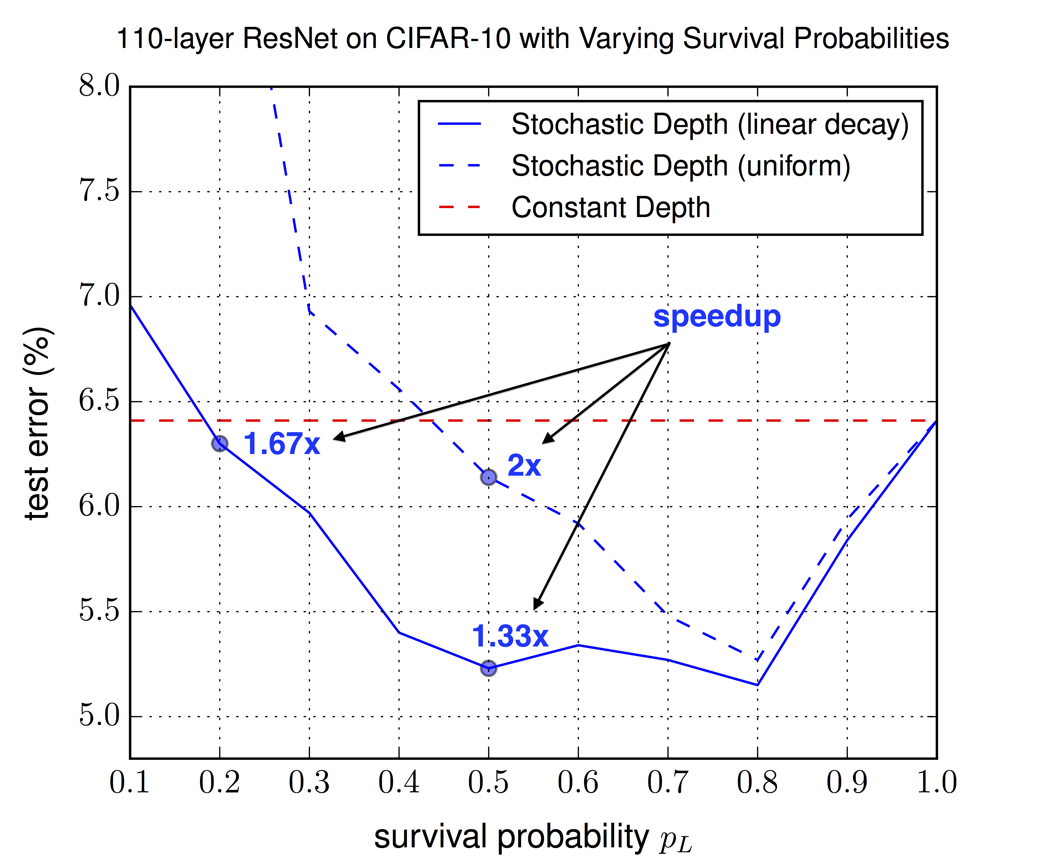
*Optimal choice of the survival probability `p_L` (in this summary `q`) for the last layer, for the uniform schema (same for all other layers) and the linear decay schema (decreasing towards `p_L`). Linear decay performs consistently better and allows for lower `p_L` values, leading to more speedup.*


--------------------

### Rough chapter-wise notes

* (1) Introduction
  * Problems of deep networks:
    * Vanishing Gradients: During backpropagation, gradients approach zero due to being repeatedly multiplied with small weights. Possible counter-measures: Careful initialization of weights, "hidden layer supervision" (?), batch normalization.
    * Diminishing feature reuse: Aequivalent problem to vanishing gradients during forward propagation. Results of early layers are repeatedly multiplied with later layer's (randomly initialized) weights. The total result then becomes meaningless noise and doesn't have a clear/strong gradient to fix it.
    * Long training time: The time of each forward-backward increases linearly with layer depth. Current 152-layer networks can take weeks to train on ImageNet.
  * I.e.: Shallow networks can be trained effectively and fast, but deep networks would be much more expressive.
  * During testing we want deep networks, during training we want shallow networks.
  * They randomly "drop out" (i.e. remove) complete layers during training (per minibatch), resulting in shallow networks.
  * Result: Lower training time *and* lower test error.
  * While dropout randomly removes width from the network, stochastic depth randomly removes depth from the networks.
  * While dropout can be thought of as training an ensemble of networks with different depth, stochastic depth can be thought of as training an ensemble of networks with different depth.
  * Stochastic depth acts as a regularizer, similar to dropout and batch normalization. It allows deeper networks without overfitting (because 1000 layers clearly wasn't enough!).

* (2) Background
  * Some previous methods to train deep networks: Greedy layer-wise training, careful initializations, batch normalization, highway connections, residual connections.
  * <Standard explanation of residual networks>
  * <Standard explanation of dropout>
  * Dropout loses effectiveness when combined with batch normalization. Seems to have basically no benefit any more for deep residual networks with batch normalization.

* (3) Deep Networks with Stochastic Depth
  * They randomly skip entire layers during training.
  * To do that, they use residual connections. They select random layers and use only the identity function for these layers (instead of the full residual block of identity + convolutions + add).
  * ResNet architecture: They use standard residual connections. ReLU activations, 2 convolutional layers (conv->BN->ReLU->conv->BN->add->ReLU). They use <= 64 filters per conv layer.
  * While the standard formula for residual connections is `output = ReLU(f(input) + identity(input))`, their formula is `output = ReLU(b * f(input) + identity(input))` with `b` being either 0 (inactive/removed layer) or 1 (active layer), i.e. is a sample of a bernoulli random variable.
  * The probabilities of the bernoulli random variables are now hyperparameters, similar to dropout.
  * Note that the probability here means the probability of *survival*, i.e. high value = more survivors.
  * The probabilities could be set uniformly, e.g. to 0.5 for each variable/layer.
  * They can also be set with a linear decay, so that the first layer has a very high probability of survival, while the last layer has a very low probability of survival.
  * Linear decay formula: `p = 1 - (l/L)(1-q)` where `l` is the current layer's number, `L` is the total number of layers, `p` is the survival probability of layer `l` and `q` is the desired survival probability of the last layer (e.g. 0.5).
  * They argue that linear decay is better, as the early layer extract low level features and are therefor more important.
  * The expected number of surviving layers is simply the sum of the probabilities.
  * For linear decay with `q=0.5` and `L=54` (i.e. 54 residual blocks = 110 total layers) the expected number of surviving blocks is roughly `(3/4)L = (3/4)54 = 40`, i.e. on average 14 residual blocks will be removed per training batch.
  * With linear decay and `q=0.5` the expected speedup of training is about 25%. `q=0.2` leads to about 40% speedup (while in one test still achieving the test error of the same network without stochastic depth).
  * Depending on the `q` setting, they observe significantly lower test errors. They argue that stochastic depth has a regularizing effect (training an ensemble of many networks with different depths).
  * Similar to dropout, the forward pass rule during testing must be slightly changed, because the network was trained on missing values. The residual formular during test time becomes `output = ReLU(p * f(input) + input)` where `p` is the average probability with which this residual block survives during training.

* (4) Results
  * Their model architecture:
    * Three chains of 18 residual blocks each, so 3*18 blocks per model.
    * Number of filters per conv. layer: 16 (first chain), 32 (second chain), 64 (third chain)
    * Between each block they use average pooling. Then they zero-pad the new dimensions (e.g. from 16 to 32 at the end of the first chain).
  * CIFAR-10:
    * Trained with SGD (momentum=0.9, dampening=0, lr=0.1 after 1st epoch, 0.01 after epoch 250, 0.001 after epoch 375).
    * Weight decay/L2 of 1e-4.
    * Batch size 128.
    * Augmentation: Horizontal flipping, crops (4px offset).
    * They achieve 5.23% error (compared to 6.41% in the original paper about residual networks).
  * CIFAR-100:
    * Same settings as before.
    * 24.58% error with stochastic depth, 27.22% without.
  * SVHN:
    * The use both the hard and easy sub-datasets of images.
    * They preprocess to zero-mean, unit-variance.
    * Batch size 128.
    * Learning rate is 0.1 (start), 0.01 (after epoch 30), 0.001 (after epoch 35).
    * 1.75% error with stochastic depth, 2.01% error without.
    * Network without stochastic depth starts to overfit towards the end.
  * Stochastic depth with linear decay and `q=0.5` gives ~25% speedup.
  * 1202-layer CIFAR-10:
    * They trained a 1202-layer deep network on CIFAR-10 (previous tests: 152 layers).
    * Without stochastic depth: 6.72% test error.
    * With stochastic depth: 4.91% test error.

* (5) Analytic experiments
  * Vanishing Gradient:
    * They analyzed the gradient that reaches the first layer.
    * The gradient with stochastic depth is consistently higher (throughout the epochs) than without stochastic depth.
    * The difference is very significant after decreasing the learning rate.
  * Hyper-parameter sensitivity:
    * They evaluated with test error for different choices of the survival probability `q`.
    * Linear decay schema: Values between 0.4 and 0.8 perform best. 0.5 is suggested (nearly best value, good spedup). Even 0.2 improves the test error (compared to no stochastic depth).
    * Uniform schema: 0.8 performs best, other values mostly significantly worse.
    * Linear decay performs consistently better than the uniform schema.

  * They define four subtasks of image understanding:
    * *Classification*: Assign a single label to a whole image.
    * *Captioning*: Assign a sequence of words (description) to a whole image*
    * *Detection*: Find objects/regions in an image and assign a single label to each one.
    * *Dense Captioning*: Find objects/regions in an image and assign a sequence of words (description) to each one.
  * DenseCap accomplishes the fourth task, i.e. it is a model that finds objects/regions in images and describes them with natural language.

### How
  * Their model consists of four subcomponents, which run for each image in sequence:
    * (1) **Convolutional Network**:
      * Basically just VGG-16.
    * (2) **Localization Layer**:
      * This layer uses a convolutional network that has mostly the same architecture as in the "Faster R-CNN" paper.
      * That ConvNet is applied to a grid of anchor points on the image.
      * For each anchor point, it extracts the features generated by the VGG-Net (model 1) around that point.
      * It then generates the attributes of `k` (default: 12) boxes using a shallow convolutional net. These attributes are (roughly): Height, width, center x, center y, confidence score.
      * It then extracts the features of these boxes from the VGG-Net output (model 1) and uses bilinear sampling to project them onto a fixed size (height, width) for the next model. The result are the final region proposals.
      * By default every image pixel is an anchor point, which results in a large number of regions. Hence, subsampling is used during training and testing.
    * (3) **Recognition Network**:
      * Takes a region (flattened to 1d vector) and projects it onto a vector of length 4096.
      * It uses fully connected layers to do that (ReLU, dropout).
      * Additionally, the network takes the 4096 vector and outputs new values for the region's position and confidence (for late fine tuning).
      * The 4096 vectors of all regions are combined to a matrix that is fed into the next component (RNN).
      * The intended sense of the this component seems to be to convert the "visual" features of each region to a more abstract, high-dimensional representation/description.
    * (4) **RNN Language Model**:
      * The take each 4096 vector and apply a fully connected layer + ReLU to it.
      * Then they feed it into an LSTM, followed by a START token.
      * The LSTM then generates word (as one hot vectors), which are fed back into the model for the next time step.
      * This is continued until the LSTM generates an END token.
  * Their full loss function has five components:
    * Binary logistic loss for the confidence values generated by the localization layer.
    * Binary logistic loss for the confidence values generated by the recognition layer.
    * Smooth L1 loss for the region dimensions generated by the localization layer.
    * Smooth L1 loss for the region dimensiosn generated by the recognition layer.
    * Cross-entropy at every time-step of the language model.
  * The whole model can be trained end-to-end.

* Results
  * They mostly use the Visual Genome dataset.
  * Their model finds lots of good regions in images.
  * Their model generates good captions for each region. (Only short captions with simple language however.)
  * The model seems to love colors. Like 30-50% of all captions contain a color. (Probably caused by the dataset?)
  * They compare to EdgeBoxes (other method to find regions in images). Their model seems to perform better.
  * Their model requires about 240ms per image (test time).
  * The generated regions and captions enable one to search for specific objects in images using text queries.


![Architecture](https://raw.githubusercontent.com/aleju/papers/master/neural-nets/images/DenseCap__architecture.png?raw=true "Architecture.")

*Architecture of the whole model. It starts with the VGG-Net ("CNN"), followed by the localization layer, which generates region proposals. Then the recognition network converts the regions to abstract high-dimensional representations. Then the language model ("RNN") generates the caption.*


![Elephant image with dense captioning.](https://raw.githubusercontent.com/aleju/papers/master/neural-nets/images/DenseCap__elephant.png?raw=true "Elephant image with dense captioning.")

![Airplane image with dense captioning.](https://raw.githubusercontent.com/aleju/papers/master/neural-nets/images/DenseCap__airplane.png?raw=true "Airplane image with dense captioning.")


--------------------

### Rough chapter-wise notes

* (1) Introduction
  * They define four subtasks of visual scene understanding:
    * Classification: Assign a single label to a whole image
    * Captioning: Assign a sequence of words (description) to a whole image
    * Detection: Find objects in an image and assign a single label to each one
    * Dense Captioning: Find objects in an image and assign a sequence of words (description) to each one
  * They developed a model for dense captioning.
  * It has two three important components:
    * A convoltional network for scene understanding
    * A localization layer for region level predictions. It predicts regions of interest and then uses bilinear sampling to extract the activations of these regions.
    * A recurrent network as the language model
  * They evaluate the model on the large-scale Visual Genome dataset (94k images, 4.1M region captions).

* (3) Model
  * Model architecture
    * Convolutional Network
      * They use VGG-16, but remove the last pooling layer.
      * For an image of size W, H the output is 512xW/16xH/16.
      * That output is the input into the localization layer.
    * Fully Convolutional Localization Layer
      * Input to this layer: Activations from the convolutional network.
      * Output of this layer: Regions of interest, as fixed-sized representations.
        * For B Regions:
          * Coordinates of the bounding boxes (matrix of shape Bx4)
          * Confidence scores (vector of length B)
          * Features (matrix of shape BxCxXxY)
      * Method: Faster R-CNN (pooling replaced by bilinear interpolation)
      * This layer is fully differentiable.
      * The localization layer predicts boxes at anchor points.
      * At each anchor point it proposes `k` boxes using a small convolutional network. It assigns a confidence score and coordinates (center x, center y, height, width) to each proposal.
      * For an image with size 720x540 and k=12 the model would have to predict 17,280 boxes, hence subsampling is used.
      * During training they use minibatches with 256/2 positive and 256/2 negative region examples. A box counts as a positive example for a specific image if it has high overlap (intersection) with an annotated box for that image.
      * During test time they use greedy non-maximum suppression (NMS) (?) to subsample the 300 most confident boxes.
      * The region proposals have varying box sizes, but the output of the localization layer (which will be fed into the RNN) is ought to have fixed sizes.
      * So they project each proposed region onto a fixed sized region. They use bilinear sampling for that projection, which is differentiable.
    * Recognition network
      * Each region is flattened to a one-dimensional vector.
      * That vector is fed through 2 fully connected layers (unknown size, ReLU, dropout), ending with a 4096 neuron layer.
      * The confidence score and box coordinates are also adjusted by the network during that process (fine tuning).
    * RNN Language Model
      * Each region is translated to a sentence.
      * The region is fed into an LSTM (after a linear layer + ReLU), followed by a special START token.
      * The LSTM outputs multiple words as one-hot-vectors, where each vector has the length `V+1` (i.e. vocabulary size + END token).
      * Loss function is average crossentropy between output words and target words.
      * During test time, words are sampled until an END tag is generated.
  * Loss function
    * Their full loss function has five components:
      * Binary logistic loss for the confidence values generated by the localization layer.
      * Binary logistic loss for the confidence values generated by the recognition layer.
      * Smooth L1 loss for the region dimensions generated by the localization layer.
      * Smooth L1 loss for the region dimensiosn generated by the recognition layer.
      * Cross-entropy at every time-step of the language model.
    * The language model term has a weight of 1.0, all other components have a weight of 0.1.
  * Training an optimization
    * Initialization: CNN pretrained on ImageNet, all other weights from `N(0, 0.01)`.
    * SGD for the CNN (lr=?, momentum=0.9)
    * Adam everywhere else (lr=1e-6, beta1=0.9, beta2=0.99)
    * CNN is trained after epoch 1. CNN's first four layers are not trained.
    * Batch size is 1.
    * Image size is 720 on the longest side.
    * They use Torch.
    * 3 days of training time.

* (4) Experiments
  * They use the Visual Genome Dataset (94k images, 4.1M regions with captions)
  * Their total vocabulary size is 10,497 words. (Rare words in captions were replaced with `<UNK>`.)
  * They throw away annotations with too many words as well as images with too few/too many regions.
  * They merge heavily overlapping regions to single regions with multiple captions.
  * Dense Captioning
    * Dense captioning task: The model receives one image and produces a set of regions, each having a caption and a confidence score.
    * Evaluation metrics
      * Evaluation of the output is non-trivial.
      * They compare predicted regions with regions from the annotation that have high overlap (above a threshold).
      * They then compare the predicted caption with the captions having similar METEOR score (above a threshold).
      * Instead of setting one threshold for each comparison they use multiple thresholds. Then they calculate the Mean Average Precision using the various pairs of thresholds.
    * Baseline models
      * Sources of region proposals during test time:
        * GT: Ground truth boxes (i.e. found by humans).
        * EB: EdgeBox (completely separate and pretrained system).
        * RPN: Their localization and recognition networks trained separately on VG regions dataset (i.e. trained without the RNN language model).
      * Models:
        * Region RNN model: Apparently the recognition layer and the RNN language model, trained on predefined regions. (Where do these regions come from? VG training dataset?)
        * Full Image RNN model: Apparently the recognition layer and the RNN language model, trained on full images from MSCOCO instead of small regions.
        * FCLN on EB: Apparently the recognition layer and the RNN language model, trained on regions generated by EdgeBox (EB) (on VG dataset?).
        * FCLN: Apparently their full model (trained on VG dataset?).
    * Discrepancy between region and image level statistics
      * When evaluating the models only on METEOR (language "quality"), the *Region RNN model* consistently outperforms the *Full Image RNN model*.
      * That's probably because the *Full Image RNN model* was trained on captions of whole images, while the *Region RNN model* was trained on captions of small regions, which tend to be a bit different from full image captions.
    * RPN outperforms external region proposals
      * Generating region proposals via RPN basically always beats EB.
    * Our model outperforms individual region description
      * Their full jointly trained model (FCLN) achieves the best results.
      * The full jointly trained model performs significantly better than `RPN + Region RNN model` (i.e. separately trained region proposal and region captioning networks).
    * Qualitative results
      * Finds plenty of good regions and generates reasonable captions for them.
      * Sometimes finds the same region twice.
    * Runtime evaluation
      * 240ms on 720x600 image with 300 region proposals.
      * 166ms on 720x600 image with 100 region proposals.
      * Recognition of region proposals takes up most time.
      * Generating region proposals takes up the 2nd most time.
      * Generating captions for regions (RNN) takes almost no time.
  * Image Retrieval using Regions and Captions
    * They try to search for regions based on search queries.
    * They search by letting their FCLN network or EB generate 100 region proposals per network. Then they calculate per region the probability of generating the search query as the caption. They use that probability to rank the results.
    * They pick images from the VG dataset, then pick captions within those images as search query. Then they evaluate the ranking of those images for the respective search query.
    * The results show that the model can learn to rank objects, object parts, people and actions as expected/desired.
    * The method described can also be used to detect an arbitrary number of distinct classes in images (as opposed to the usual 10 to 1000 classes), because the classes are contained in the generated captions.

  * The authors train a variant of AlexNet that has significantly fewer parameters than the original network, while keeping the network's accuracy stable.
  * Advantages of this:
    * More efficient distributed training, because less parameters have to be transferred.
    * More efficient transfer via the internet, because the model's file size is smaller.
    * Possibly less memory demand in production, because fewer parameters have to be kept in memory.

### How
  * They define a Fire Module. A Fire Module contains of:
    * Squeeze Module: A 1x1 convolution that reduces the number of channels (e.g. from 128x32x32 to 64x32x32).
    * Expand Module: A 1x1 convolution and a 3x3 convolution, both applied to the output of the Squeeze Module. Their results are concatenated.
  * Using many 1x1 convolutions is advantageous, because they need less parameters than 3x3s.
  * They use ReLUs, only convolutions (no fully connected layers) and Dropout (50%, before the last convolution).
  * They use late maxpooling. They argue that applying pooling late - rather than early - improves accuracy while not needing more parameters.
  * They try residual connections:
    * One network without any residual connections (performed the worst).
    * One network with residual connections based on identity functions, but only between layers of same dimensionality (performed the best).
    * One network with residual connections based on identity functions and other residual connections with 1x1 convs (where dimensionality changed) (performance between the other two).
  * They use pruning from Deep Compression to reduce the parameters further. Pruning simply collects the 50% of all parameters of a layer that have the lowest values and sets them to zero. That creates a sparse matrix.

### Results
  * 50x parameter reduction of AlexNet (1.2M parameters before pruning, 0.4M after pruning).
  * 510x file size reduction of AlexNet (from 250mb to 0.47mb) when combined with Deep Compression.
  * Top-1 accuracy remained stable.
  * Pruning apparently can be used safely, even after the network parameters have already been reduced significantly.
  * While pruning was generally safe, they found that two of their later layers reacted quite sensitive to it. Adding parameters to these (instead of removing them) actually significantly improved accuracy.
  * Generally they found 1x1 convs to react more sensitive to pruning than 3x3s. Therefore they focused pruning on 3x3 convs.
  * First pruning a network, then re-adding the pruned weights (initialized with 0s) and then retraining for some time significantly improved accuracy.
  * The network was rather resilient to significant channel reduction in the Squeeze Modules. Reducing to 25-50% of the original channels (e.g. 128x32x32 to 64x32x32) seemed to be a good choice.
  * The network was rather resilient to removing 3x3 convs and replacing them with 1x1 convs. A ratio of 2:1 to 1:1 (1x1 to 3x3) seemed to produce good results while mostly keeping the accuracy.
  * Adding some residual connections between the Fire Modules improved the accuracy.
  * Adding residual connections with identity functions *and also* residual connections with 1x1 convs (where dimensionality changed) improved the accuracy, but not as much as using *only* residual connections with identity functions (i.e. it's better to keep some modules without identity functions).


--------------------

### Rough chapter-wise notes

* (1) Introduction and Motivation
  * Advantages from having less parameters:
    * More efficient distributed training, because less data (parameters) have to be transfered.
    * Less data to transfer to clients, e.g. when a model used by some app is updated.
    * FPGAs often have hardly any memory, i.e. a model has to be small to be executed.
  * Target here: Find a CNN architecture with less parameters than an existing one but comparable accuracy.

* (2) Related Work
  * (2.1) Model Compression
    * SVD-method: Just apply SVD to the parameters of an existing model.
    * Network Pruning: Replace parameters below threshold with zeros (-> sparse matrix), then retrain a bit.
    * Add quantization and huffman encoding to network pruning = Deep Compression.
  * (2.2) CNN Microarchitecture
    * The term "CNN Microarchitecture" refers to the "organization and dimensions of the individual modules" (so an Inception module would have a complex CNN microarchitecture).
  * (2.3) CNN Macroarchitecture
    * CNN Macroarchitecture = "big picture" / organization of many modules in a network / general characteristics of the network, like depth
    * Adding connections between modules can help (e.g. residual networks)
  * (2.4) Neural Network Design Space Exploration
    * Approaches for Design Space Exporation (DSE):
      * Bayesian Optimization, Simulated Annealing, Randomized Search, Genetic Algorithms

* (3) SqueezeNet: preserving accuracy with few parameters
  * (3.1) Architectural Design Strategies
    * A conv layer with N filters applied to CxHxW input (e.g. 3x128x128 for a possible first layer) with kernel size kHxkW (e.g. 3x3) has `N*C*kH*kW` parameters.
    * So one way to reduce the parameters is to decrease kH and kW, e.g. from 3x3 to 1x1 (reduces parameters by a factor of 9).
    * A second way is to reduce the number of channels (C), e.g. by using 1x1 convs before the 3x3 ones.
    * They think that accuracy can be improved by performing downsampling later in the network (if parameter count is kept constant).
  * (3.2) The Fire Module
    * The Fire Module has two components:
      * Squeeze Module:
        * One layer of 1x1 convs
      * Expand Module:
        * Concat the results of:
          * One layer of 1x1 convs
          * One layer of 3x3 convs
    * The Squeeze Module decreases the number of input channels significantly.
    * The Expand Module then increases the number of input channels again.
  * (3.3) The SqueezeNet architecture
    * One standalone conv, then several fire modules, then a standalone conv, then global average pooling, then softmax.
    * Three late max pooling laters.
    * Gradual increase of filter numbers.
    * (3.3.1) Other SqueezeNet details
      * ReLU activations
      * Dropout before the last conv layer.
      * No linear layers.

* (4) Evaluation of SqueezeNet
  * Results of competing methods:
    * SVD: 5x compression, 56% top-1 accuracy
    * Pruning: 9x compression, 57.2% top-1 accuracy
    * Deep Compression: 35x compression, ~57% top-1 accuracy
  * SqueezeNet: 50x compression, ~57% top-1 accuracy
  * SqueezeNet combines low parameter counts with Deep Compression.
  * The accuracy does not go down because of that, i.e. apparently Deep Compression can even be applied to small models without giving up on performance.

* (5) CNN Microarchitecture Design Space Exploration
  * (5.1) CNN Microarchitecture metaparameters
    * blabla we test various values for this and that parameter
  * (5.2) Squeeze Ratio
    * In a Fire Module there is first a Squeeze Module and then an Expand Module. The Squeeze Module decreases the number of input channels to which 1x1 and 3x3 both are applied (at the same time).
    * They analyzed how far you can go down with the Sqeeze Module by training multiple networks and calculating the top-5 accuracy for each of them.
    * The accuracy by Squeeze Ratio (percentage of input channels kept in 1x1 squeeze, i.e. 50% = reduced by half, e.g. from 128 to 64):
      * 12%: ~80% top-5 accuracy
      * 25%: ~82% top-5 accuracy
      * 50%: ~85% top-5 accuracy
      * 75%: ~86% top-5 accuracy
      * 100%: ~86% top-5 accuracy
  * (5.3) Trading off 1x1 and 3x3 filters
    * Similar to the Squeeze Ratio, they analyze the optimal ratio of 1x1 filters to 3x3 filters.
    * E.g. 50% would mean that half of all filters in each Fire Module are 1x1 filters.
    * Results:
      * 01%: ~76% top-5 accuracy
      * 12%: ~80% top-5 accuracy
      * 25%: ~82% top-5 accuracy
      * 50%: ~85% top-5 accuracy
      * 75%: ~85% top-5 accuracy
      * 99%: ~85% top-5 accuracy

* (6) CNN Macroarchitecture Design Space Exploration
  * They compare the following networks:
    * (1) Without residual connections
    * (2) With residual connections between modules of same dimensionality
    * (3) With residual connections between all modules (except pooling layers) using 1x1 convs (instead of identity functions) where needed
  * Adding residual connections (2) improved top-1 accuracy from 57.5% to 60.4% without any new parameters.
  * Adding complex residual connections (3) worsed top-1 accuracy again to 58.8%, while adding new parameters.

* (7) Model Compression Design Space Exploration
  * (7.1) Sensitivity Analysis: Where to Prune or Add parameters
    * They went through all layers (including each one in the Fire Modules).
    * In each layer they set the 50% smallest weights to zero (pruning) and measured the effect on the top-5 accuracy.
    * It turns out that doing that has basically no influence on the top-5 accuracy in most layers.
    * Two layers towards the end however had significant influence (accuracy went down by 5-10%).
    * Adding parameters to these layers improved top-1 accuracy from 57.5% to 59.5%.
    * Generally they found 1x1 layers to be more sensitive than 3x3 layers so they pruned them less aggressively.
  * (7.2) Improving Accuracy by Densifying Sparse Models
    * They found that first pruning a model and then retraining it again (initializing the pruned weights to 0) leads to higher accuracy.
    * They could improve top-1 accuracy by 4.3% in this way.

  * AIR (attend, infer, repeat) is a recurrent autoencoder architecture to transform images into latent representations object by object.
  * As an autoencoder it is unsupervised.
  * The latent representation is generated in multiple time steps.
  * Each time step is intended to encode information about exactly one object in the image.
  * The information encoded for each object is (mostly) a what-where information, i.e. which class the object has and where (in 2D: translation, scaling) it is shown.
  * AIR has a dynamic number of time step. After encoding one object the model can decide whether it has encoded all objects or whether there is another one to encode. As a result the latent layer size is not fixed.
  * AIR uses an attention mechanism during the encoding to focus on each object.

### How
  * At its core, AIR is a variational autoencoder.
  * It maximizes lower bounds on the error instead of using a "classic" reconstruction error (like MSE on the euclidean distance).
  * It has an encoder and a decoder.
  * The model uses a recurrent architecture via an LSTM.
  * It (ideally) encodes/decodes one object per time step.
  * Encoder
    * The encoder receives the image and generates latent information for one object (what object, where it is).
    * At the second timestep it receives the image, the previous timestep's latent information and the previous timestep's hidden layer. It then generates another latent information (for another object).
    * And so on.
  * Decoder
    * The decoder receives latent information from the encoder (timestep by timestep) and treats it as a what-where information when reconstructing the images.
      * It takes the what-part and uses a "normal" decoder to generate an image that shows the object.
      * It takes the where-part and the generated image and feeds both into a spatial transformer, which then transforms the generated image by translating or rotating it.
  * Dynamic size
    * AIR makes use of a dynamically sized latent layer. It is not necessarily limited to a fixed number of time steps.
    * Implementation: Instead of just letting the encoder generate what-where information, the encoder also generates a "present" information, which is 0 or 1. If it is 1, the reccurence will continue with encoding and decoding another object. Otherwise it will stop.
  * Attention
    * To add an attention mechanism, AIR first uses the LSTM's hidden layer to generate "where" and "present" information per object.
    * It stops if the "present" information is 0.
    * Otherwise it uses the "where" information to focus on the object using a spatial transformer. The object is then encoded to the "what" information.

### Results
  * On a dataset of images, each containing multiple MNIST digits, AIR learns to accurately count the digits and estimate their position and scale.
  * When AIR is trained on images of 0 to 2 digits and tested on images containing 3 digits it performs poorly.
  * When AIR is trained on images of 0, 1 or 3 digits and tested on images containing 2 digits it performs mediocre.
  * DAIR performs well on both tasks. Likely because it learns to remove each digit from the image after it has investigated it.
  * When AIR is trained on 0 to 2 digits and a second network is trained (separately) to work with the generated latent layer (trained to sum the shown digits and rate whether they are shown in ascending order), then that second network reaches high accuracy with relatively few examples. That indicates usefulness for unsupervised learning.
  * When AIR is trained on a dataset of handwritten characters from different alphabets, it learns to represent distinct strokes in its latent layer.
  * When AIR is trained in combination with a renderer (inverse graphics), it is able to accurately recover latent parameters of rendered objects - better than supervised networks. That indicates usefulness for robots which have to interact with objects.


![Architecture](https://raw.githubusercontent.com/aleju/papers/master/neural-nets/images/Attend_Infer_Repeat__architecture.png?raw=true "Architecture.")

*AIR architecture for MNIST. Left: Decoder for two objects that are each first generated (y_att) and then fed into a Spatial Transformer (y) before being combined into an image (x). Middle: , Right: Encoder with multiple time steps that generates what-where information per object and stops when the "present" information (z_pres) is 0. Right: Combination of both for MNIST with Spatial Transformer for the attention mechanism (top left).*


![DAIR Architecture](https://raw.githubusercontent.com/aleju/papers/master/neural-nets/images/Attend_Infer_Repeat__architecture_dair.png?raw=true "DAIR Architecture.")

*Encoder with DAIR architecture. DAIR modifies the image after every timestep (e.g. to remove objects that were already encoded).*


--------------------

### Rough chapter-wise notes

* (1) Introduction
  * Assumption: Images are made up of distinct objects. These objects have visual and physical properties.
  * They developed a framework for efficient inference in images (i.e. get from the image to a latent representation of the objects, i.e. inverse graphics).
  * Parts of the framework: High dimensional representations (e.g. object images), interpretable latent variables (e.g. for rotation) and generative processes (to combine object images with latent variables).
  * Contributions:
    * A scheme for efficient variational inference in latent spaces of variable dimensionality.
      * Idea: Treat inference as an iterative process, implemented via an RNN that looks at one object at a time and learns an appropriate number of inference steps. (Attend-Infer-Repeat, AIR)
      * End-to-end training via amortized variational inference (continuous variables: gradient descent, discrete variables: black-box optimization).
    * AIR allows to train generative models that automatically learn to decompose scenes.
    * AIR allows to recover objects and their attributes from rendered 3D scenes (inverse rendering).

* (2) Approach
  * Just like in VAEs, the scene interpretation is treated with a bayesian approach.
  * There are latent variables `z` and images `x`.
  * Images are generated via a probability distribution `p(x|z)`.
  * This can be reversed via bayes rule to `p(x|z) = p(x)p(z|x) / p(z)`, which means that `p(x|z)p(z) / p(x) = p(z|x)`.
  * The prior `p(z)` must be chosen and captures assumptions about the distributions of the latent variables.
  * `p(x|z)` is the likelihood and represents the model that generates images from latent variables.
  * They assume that there can be multiple objects in an image.
  * Every object gets its own latent variables.
  * A probability distribution p(x|z) then converts each object (on its own) from the latent variables to an image.
  * The number of objects follows a probability distribution `p(n)`.
  * For the prior and likelihood they assume two scenarios:
    * 2D: Three dimensions for X, Y and scale. Additionally n dimensions for its shape.
    * 3D: Dimensions for X, Y, Z, rotation, object identity/category (multinomial variable). (No scale?)
  * Both 2D and 3D can be separated into latent variables for "where" and "what".
  * It is assumed that the prior latent variables are independent of each other.
  * (2.1) Inference
    * Inference for their model is intractable, therefore they use an approximation `q(z,n|x)`, which minizes `KL(q(z,n|x)||p(z,n|x))`, i.e. KL(approximation||real) using amortized variational approximation.
    * Challenges for them:
      * The dimensionality of their latent variable layer is a random variable p(n) (i.e. no static size.).
      * Strong symmetries.
    * They implement inference via an RNN which encodes the image object by object.
    * The encoded latent variables can be gaussians.
    * They encode the latent layer length `n` via a vector (instead of an integer). The vector has the form of `n` ones followed by one zero.
    * If the length vector is `#z` then they want to approximate `q(z,#z|x)`.
    * That can apparently be decomposed into `<product> q(latent variable value i, #z is still 1 at i|x, previous latent variable values) * q(has length n|z,x)`.
    * So instead of computing `#z` once, they instead compute at every time step whether there is another object in the image, which indirectly creates a chain of ones followed by a zero (the `#z` vector).
  * (2.2) Learning
    * The parameters theta (`p`, latent variable -> image) and phi (`q`, image -> latent variables) are jointly optimized.
    * Optimization happens by maximizing a lower bound `E[log(p(x,z,n) / q(z,n|x))]` called the negative free energy.
    * (2.2.1) Parameters of the model theta
      * Parameters theta of log(p(x,z,n)) can easily be obtained using differentiation, so long as z and n are well approximated.
      * The differentiation of the lower bound with repsect to theta can be approximated using Monte Carlo methods.
    * (2.2.2) Parameters of the inference network phi
      * phi are the parameters of q, i.e. of the RNN that generates z and #z in i timesteps.
      * At each timestep (i.e. per object) the RNN generates three kinds of information: What (object), where (it is), whether it is present (i <= n).
      * Each of these information is represented via variables. These variables can be discrete or continuous.
      * When differentiating w.r.t. a continuous variable they use the reparameterization trick.
      * When differentiating w.r.t. a discrete variable they use the likelihood ratio estimator.

* (3) Models and Experiments
  * The RNN is implemented via an LSTM.
  * DAIR
    * The "normal" AIR model uses at every time step the image and the RNN's hidden layer to generate the next latent information (what object, where it is and whether it is present).
    * DAIR uses that latent information to change the image at every time step and then use the difference (D) image for the next time step, i.e. DAIR can remove an object from the image after it has generated latent variables for it.
  * (3.1) Multi-MNIST
    * They generate a dataset of images containing multiple MNIST digits.
    * Each image contains 0 to 2 digits.
    * AIR is trained on the dataset.
    * It learns without supervision a good attention scanning policy for the images (to "hit" all digits), to count the digits visible in the image and to use a matching number of time steps.
    * During training, the model seems to first learn proper reconstruction of the digits and only then to do it with as few timesteps as possible.
    * (3.1.1) Strong Generalization
      * They test the generalization capabilities of AIR.
      * *Extrapolation task*: They generate images with 0 to 2 digits for training, then test on images with 3 digits. The model is unable to correctly count the digits (~0% accuracy).
      * *Interpolation task*: They generate images with 0, 1 or 3 digits for training, then test on images with 2 digits. The model performs OK-ish (~60% accuracy).
      * DAIR performs in both cases well (~80% for extrapolation, ~95% accuracy for interpolation).
    * (3.1.2) Representational Power
      * They train AIR on images containing 0, 1 or 2 digits.
      * Then they train a second network. That network takes the output of the first one and computes a) the sum of the digits and b) estimates whether they are shown in ascending order.
      * Accuracy for both tasks is ~95%.
      * The network reaches that accuracy significantly faster than a separately trained CNN (i.e. requires less labels / is more unsupervised).
  * (3.2) Omniglot
    * They train AIR on the Omniglot dataset (1.6k handwritten characters from 50 alphabets).
    * They allow the model to use up to 4 timesteps.
    * The model learns to reconstruct the images in timesteps that resemble strokes.
  * (3.3) 3D Scenes
    * Here, the generator p(x|z) is a 3D renderer, only q(z|x) must be approximated.
    * The model has to learn to count the objects and to estimate per object its identity (class) and pose.
    * They use "finite-differencing" to get gradients through the renderer and use "score function estimators" to get gradients with respect to discrete variables.
    * They first test with a setup where the object count is always 1. The network learns to accurately recover the object parameters.
    * A similar "normal" network has much more problems with recovering the parameters, especially rotation, because the conditional probabilities are multi-modal. The lower bound maximization strategy seems to work better in those cases.
    * In a second experiment with multiple complex objects, AIR also achieves high reconstruction accuracy.

  * They use an implementation of Q-learning (i.e. reinforcement learning) with CNNs to automatically play Atari games.
  * The algorithm receives the raw pixels as its input and has to choose buttons to press as its output. No hand-engineered features are used. So the model "sees" the game and "uses" the controller, just like a human player would.
  * The model achieves good results on various games, beating all previous techniques and sometimes even surpassing human players.

### How
  * Deep Q Learning
    * *This is yet another explanation of deep Q learning, see also [this blog post](http://www.nervanasys.com/demystifying-deep-reinforcement-learning/) for longer explanation.*
    * While playing, sequences of the form (`state1`, `action1`, `reward`, `state2`) are generated.
      * `state1` is the current game state. The agent only sees the pixels of that state. (Example: Screen shows enemy.)
      * `action1` is an action that the agent chooses. (Example: Shoot!)
      * `reward` is the direct reward received for picking `action1` in `state1`. (Example: +1 for a kill.)
      * `state2` is the next game state, after the action was chosen in `state1`. (Example: Screen shows dead enemy.)
    * One can pick actions at random for some time to generate lots of such tuples. That leads to a replay memory.
    * Direct reward
      * After playing randomly for some time, one can train a model to predict the direct reward given a screen (we don't want to use the whole state, just the pixels) and an action, i.e. `Q(screen, action) -> direct reward`.
      * That function would need a forward pass for each possible action that we could take. So for e.g. 8 buttons that would be 8 forward passes. To make things more efficient, we can let the model directly predict the direct reward for each available action, e.g. for 3 buttons `Q(screen) -> (direct reward of action1, direct reward of action2, direct reward of action3)`.
      * We can then sample examples from our replay memory. The input per example is the screen. The output is the reward as a tuple. E.g. if we picked button 1 of 3 in one example and received a reward of +1 then our output/label for that example would be `(1, 0, 0)`.
      * We can then train the model by playing completely randomly for some time, then sample some batches and train using a mean squared error. Then play a bit less randomly, i.e. start to use the action which the network thinks would generate the highest reward. Then train again, and so on.
    * Indirect reward
      * Doing the previous steps, the model will learn to anticipate the *direct* reward correctly. However, we also want it to predict indirect rewards. Otherwise, the model e.g. would never learn to shoot rockets at enemies, because the reward from killing an enemy would come many frames later.
      * To learn the indirect reward, one simply adds the reward value of highest reward action according to `Q(state2)` to the direct reward.
      * I.e. if we have a tuple (`state1`, `action1`, `reward`, `state2`), we would not add (`state1`, `action1`, `reward`) to the replay memory, but instead (`state1`, `action1`, `reward + highestReward(Q(screen2))`). (Where `highestReward()` returns the reward of the action with the highest reward according to Q().)
      * By training to predict `reward + highestReward(Q(screen2))` the network learns to anticipate the direct reward *and* the indirect reward. It takes a leap of faith to accept that this will ever converge to a good solution, but it does.
      * We then add `gamma` to the equation: `reward + gamma*highestReward(Q(screen2))`. `gamma` may be set to 0.9. It is a discount factor that devalues future states, e.g. because the world is not deterministic and therefore we can't exactly predict what's going to happen. Note that Q will automatically learn to stack it, e.g. `state3` will be discounted to `gamma^2` at `state1`.
  * This paper
    * They use the mentioned Deep Q Learning to train their model Q.
    * They use a k-th frame technique, i.e. they let the model decide upon an action at (here) every 4th frame.
    * Q is implemented via a neural net. It receives 84x84x4 grayscale pixels that show the game and projects that onto the rewards of 4 to 18 actions.
    * The input is HxWx4 because they actually feed the last 4 frames into the network, instead of just 1 frame. So the network knows more about what things are moving how.
    * The network architecture is:
      * 84x84x4 (input)
      * 16 convs, 8x8, stride 4, ReLU
      * 32 convs, 4x4, stride 2, ReLU
      * 256 fully connected neurons, ReLU
      * <N_actions> fully connected neurons, linear
    * They use a replay memory of 1 million frames.

### Results
  * They ran experiments on the Atari games Beam Rider, Breakout, Enduro, Pong, Qbert, Seaquest and Space Invaders.
  * Same architecture and hyperparameters for all games.
  * Rewards were based on score changes in the games, i.e. they used +1 (score increases) and -1 (score decreased).
  * Optimizer: RMSProp, Batch Size: 32.
  * Trained for 10 million examples/frames per game.
  * They had no problems with instability and their average Q value per game increased smoothly.
  * Their method beats all other state of the art methods.
  * They managed to beat a human player in games that required not so much "long" term strategies (the less frames the better).
  * Video: starts at 46:05. 
 https://youtu.be/dV80NAlEins?t=46m05s 


![Algorithm](https://raw.githubusercontent.com/aleju/papers/master/neural-nets/images/Playing_Atari_with_Deep_Reinforcement_Learning__algorithm.png?raw=true "Algorithm")

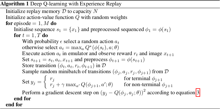
*The original full algorithm, as shown in the paper.*

--------------------

### Rough chapter-wise notes

* (1) Introduction
  * Problems when using neural nets in reinforcement learning (RL):
    * Reward signal is often sparse, noise and delayed.
    * Often assumption that data samples are independent, while they are correlated in RL.
    * Data distribution can change when the algorithm learns new behaviours.
  * They use Q-learning with a CNN and stochastic gradient descent.
  * They use an experience replay mechanism (i.e. memory) from which they can sample previous transitions (for training).
  * They apply their method to Atari 2600 games in the Arcade Learning Environment (ALE).
  * They use only the visible pixels as input to the network, i.e. no manual feature extraction.

* (2) Background
  * blablabla, standard deep q learning explanation

* (3) Related Work
  * TD-Backgammon: "Solved" backgammon. Worked similarly to Q-learning and used a multi-layer perceptron.
  * Attempts to copy TD-Backgammon to other games failed.
  * Research was focused on linear function approximators as there were problems with non-linear ones diverging.
  * Recently again interest in using neural nets for reinforcement learning. Some attempts to fix divergence problems with gradient temporal-difference methods.
  * NFQ is a very similar method (to the one in this paper), but worked on the whole batch instead of minibatches, making it slow. It also first applied dimensionality reduction via autoencoders on the images instead of training on them end-to-end.
  * HyperNEAT was applied to Atari games and evolved a neural net for each game. The networks learned to exploit design flaws.

* (4) Deep Reinforcement Learning
  * They want to connect a reinforcement learning algorithm with a deep neural network, e.g. to get rid of handcrafted features.
  * The network is supposes to run on the raw RGB images.
  * They use experience replay, i.e. store tuples of (pixels, chosen action, received reward) in a memory and use that during training.
  * They use Q-learning.
  * They use an epsilon-greedy policy.
  * Advantages from using experience replay instead of learning "live" during game playing:
    * Experiences can be reused many times (more efficient).
    * Samples are less correlated.
    * Learned parameters from one batch don't determine as much the distributions of the examples in the next batch.
  * They save the last N experiences and sample uniformly from them during training.
  * (4.1) Preprocessing and Model Architecture
    * Raw Atari images are 210x160 pixels with 128 possible colors.
    * They downsample them to 110x84 pixels and then crop the 84x84 playing area out of them.
    * They also convert the images to grayscale.
    * They use the last 4 frames as input and stack them.
    * So their network input has shape 84x84x4.
    * They use one output neuron per possible action. So they can compute the Q-value (expected reward) of each action with one forward pass.
    * Architecture: 84x84x4 (input) => 16 8x8 convs, stride 4, ReLU => 32 4x4 convs stride 2 ReLU => fc 256, ReLU => fc N actions, linear
    * 4 to 18 actions/outputs (depends on the game).
    * Aside from the outputs, the architecture is the same for all games.

* (5) Experiments
  * Games that they played: Beam Rider, Breakout, Enduro, Pong, Qbert, Seaquest, Space Invaders
  * They use the same architecture und hyperparameters for all games.
  * They give a reward of +1 whenever the in-game score increases and -1 whenever it decreases.
  * They use RMSProp.
  * Mini batch size was 32.
  * They train for 10 million frames/examples.
  * They initialize epsilon (in their epsilon greedy strategy) to 1.0 and decrease it linearly to 0.1 at one million frames.
  * They let the agent decide upon an action at every 4th in-game frame (3rd in space invaders).
  * (5.1) Training and stability
    * They plot the average reward und Q-value per N games to evaluate the agent's training progress,
    * The average reward increases in a noisy way.
    * The average Q value increases smoothly.
    * They did not experience any divergence issues during their training.
  * (5.2) Visualizating the Value Function
    * The agent learns to predict the value function accurately, even for rather long sequences (here: ~25 frames).
  * (5.3) Main Evaluation
    * They compare to three other methods that use hand-engineered features and/or use the pixel data combined with significant prior knownledge.
    * They mostly outperform the other methods.
    * They managed to beat a human player in three games. The ones where the human won seemed to require strategies that stretched over longer time frames.