* Traditionally neural nets use max pooling with 2x2 grids (2MP).
  * 2MP reduces the image dimensions by a factor of 2.
  * An alternative would be to use pooling schemes that reduce by factors other than two, e.g. `1 < factor < 2`.
  * Pooling by a factor of `sqrt(2)` would allow twice as many pooling layers as 2MP, resulting in "softer" image size reduction throughout the network.
  * Fractional Max Pooling (FMP) is such a method to perform max pooling by factors other than 2.

### How
  * In 2MP you move a 2x2 grid always by 2 pixels.
  * Imagine that these step sizes follow a sequence, i.e. for 2MP: `2222222...`
  * If you mix in just a single `1` you get a pooling factor of `<2`.
  * By chosing the right amount of `1s` vs. `2s` you can pool by any factor between 1 and 2.
  * The sequences of `1s` and `2s` can be generated in fully *random* order or in *pseudorandom* order, where pseudorandom basically means "predictable sub patterns" (e.g. 211211211211211...).
  * FMP can happen *disjoint* or *overlapping*. Disjoint means 2x2 grids, overlapping means 3x3.

### Results
  * FMP seems to perform generally better than 2MP.
  * Better results on various tests, including CIFAR-10 and CIFAR-100 (often quite significant improvement).
  * Best configuration seems to be *random* sequences with *overlapping* regions.
  * Results are especially better if each test is repeated multiple times per image (as the random sequence generation creates randomness, similar to dropout). First 5-10 repetitions seem to be most valuable, but even 100+ give some improvement.
  * An FMP-factor of `sqrt(2)` was usually used.


![Examples](https://raw.githubusercontent.com/aleju/papers/master/neural-nets/images/Fractional_Max_Pooling__examples.jpg?raw=true "Examples")

*Random FMP with a factor of sqrt(2) applied five times to the same input image (results upscaled back to original size).*

-------------------------

### Rough chapter-wise notes

* (1) Convolutional neural networks
  * Advantages of 2x2 max pooling (2MP): fast; a bit invariant to translations and distortions; quick reduction of image sizes
  * Disadvantages: "disjoint nature of pooling regions" can limit generalization (i.e. that they don't overlap?); reduction of image sizes can be too quick
  * Alternatives to 2MP: 3x3 pooling with stride 2, stochastic 2x2 pooling
  * All suggested alternatives to 2MP also reduce sizes by a factor of 2
  * Author wants to have reduction by sqrt(2) as that would enable to use twice as many pooling layers
  * Fractional Max Pooling = Pooling that reduces image sizes by a factor of `1 < alpha < 2`
  * FMP introduces randomness into pooling (by the choice of pooling regions)
  * Settings of FMP:
    * Pooling Factor `alpha` in range [1, 2] (1 = no change in image sizes, 2 = image sizes get halfed)
    * Choice of Pooling-Regions: Random or pseudorandom. Random is stronger (?). Random+Dropout can result in underfitting.
    * Disjoint or overlapping pooling regions. Results for overlapping are better.

* (2) Fractional max-pooling
  * For traditional 2MP, every grid's top left coordinate is at `(2i-1, 2j-1)` and it's bottom right coordinate at `(2i, 2j)` (i=col, j=row).
  * It will reduce the original size N to 1/2N, i.e. `2N_in = N_out`.
  * Paper analyzes `1 < alpha < 2`, but `alpha > 2` is also possible.
  * Grid top left positions can be described by sequences of integers, e.g. (only column): 1, 3, 5, ...
  * Disjoint 2x2 pooling might be 1, 3, 5, ... while overlapping would have the same sequence with a larger 3x3 grid.
  * The increment of the sequences can be random or pseudorandom for alphas < 2.
  * For 2x2 FMP you can represent any alpha with a "good" sequence of increments that all have values `1` or `2`, e.g. 2111121122111121...
  * In the case of random FMP, the optimal fraction of 1s and 2s is calculated. Then a random permutation of a sequence of 1s and 2s is generated.
  * In the case of pseudorandom FMP, the 1s and 2s follow a pattern that leads to the correct alpha, e.g. 112112121121211212...
  * Random FMP creates varying distortions of the input image. Pseudorandom FMP is a faithful downscaling.
 
* (3) Implementation
  * In their tests they use a convnet starting with 10 convolutions, then 20, then 30, ...
  * They add FMP with an alpha of sqrt(2) after every conv layer.
  * They calculate the desired output size, then go backwards through their network to the input. They multiply the size of the image by sqrt(2) with every FMP layer and add a flat 1 for every conv layer. The result is the required image size. They pad the images to that size.
  * They use dropout, with increasing strength from 0% to 50% towards the output.
  * They use LeakyReLUs.
  * Every time they apply an FMP layer, they generate a new sequence of 1s and 2s. That indirectly makes the network an ensemble of similar networks.
  * The output of the network can be averaged over several forward passes (for the same image). The result then becomes more accurate (especially up to >=6 forward passes).

* (4) Results
  * Tested on MNIST and CIFAR-100
  * Architectures (somehow different from (3)?):
    * MNIST: 36x36 img -> 6 times (32 conv (3x3?) -> FMP alpha=sqrt(2)) -> ? -> ? -> output
    * CIFAR-100: 94x94 img -> 12 times (64 conv (3x3?) -> FMP alpha=2^(1/3)) -> ? -> ? -> output
  * Overlapping pooling regions seemed to perform better than disjoint regions.
  * Random FMP seemed to perform better than pseudorandom FMP.
  * Other tests:
    * "The Online Handwritten Assamese Characters Dataset": FMP performed better than 2MP (though their network architecture seemed to have significantly more parameters
    * "CASIA-OLHWDB1.1 database": FMP performed better than 2MP (again, seemed to have more parameters)
    * CIFAR-10: FMP performed better than current best network (especially with many tests per image)

  * Inception v4 is like Inception v3, but
    * Slimmed down, i.e. some parts were simplified
    * One new version with residual connections (Inception-ResNet-v2), one without (Inception-v4)
  * They didn't observe an improved error rate when using residual connections.
  * They did however oberserve that using residual connections decreased their training times.
  * They had to scale down the results of their residual modules (multiply them by a constant ~0.1). Otherwise their networks would die (only produce 0s).
  * Results on ILSVRC 2012 (val set, 144 crops/image):
    * Top-1 Error:
      * Inception-v4: 17.7%
      * Inception-ResNet-v2: 17.8%
    * Top-5 Error (ILSVRC 2012 val set, 144 crops/image):
      * Inception-v4: 3.8%
      * Inception-ResNet-v2: 3.7% 

### Architecture
  * Basic structure of Inception-ResNet-v2 (layers, dimensions):
    * `Image -> Stem -> 5x Module A -> Reduction-A -> 10x Module B -> Reduction B -> 5x Module C -> AveragePooling -> Droput 20% -> Linear, Softmax`
    * `299x299x3 -> 35x35x256 -> 35x35x256 -> 17x17x896 -> 17x17x896 -> 8x8x1792 -> 8x8x1792 -> 1792 -> 1792 -> 1000`
  * Modules A, B, C are very similar.
  * They contain 2 (B, C) or 3 (A) branches.
  * Each branch starts with a 1x1 convolution on the input.
  * All branches merge into one 1x1 convolution (which is then added to the original input, as usually in residual architectures).
  * Module A uses 3x3 convolutions, B 7x1 and 1x7, C 3x1 and 1x3.
  * The reduction modules also contain multiple branches. One has max pooling (3x3 stride 2), the other branches end in convolutions with stride 2.

![Module A](https://raw.githubusercontent.com/aleju/papers/master/neural-nets/images/Inception_v4__module_a.png?raw=true "Module A")
![Module B](https://raw.githubusercontent.com/aleju/papers/master/neural-nets/images/Inception_v4__module_b.png?raw=true "Module B")
![Module C](https://raw.githubusercontent.com/aleju/papers/master/neural-nets/images/Inception_v4__module_c.png?raw=true "Module C")
![Reduction Module A](https://raw.githubusercontent.com/aleju/papers/master/neural-nets/images/Inception_v4__reduction_a.png?raw=true "Reduction Module A")

*From top to bottom: Module A, Module B, Module C, Reduction Module A.*

![Top 5 error](https://raw.githubusercontent.com/aleju/papers/master/neural-nets/images/Inception_v4__top5_error.png?raw=true "Top 5 error")

*Top 5 eror by epoch, models with (red, solid, bottom) and without (green, dashed) residual connections.*

-------------------------

### Rough chapter-wise notes

### Introduction, Related Work
  * Inception v3 was adapted to run on DistBelief. Inception v4 is designed for TensorFlow, which gets rid of some constraints and allows a simplified architecture.
  * Authors don't think that residual connections are inherently needed to train deep nets, but they do speed up the training.
  * History:
    * Inception v1 - Introduced inception blocks
    * Inception v2 - Added Batch Normalization
    * Inception v3 - Factorized the inception blocks further (more submodules)
    * Inception v4 - Adds residual connections

### Architectural Choices
  * Previous architectures were constrained due to memory problems. TensorFlow got rid of that problem.
  * Previous architectures were carefully/conservatively extended. Architectures ended up being quite complicated. This version slims down everything.
  * They had problems with residual networks dieing when they contained more than 1000 filters (per inception module apparently?). They could fix that by multiplying the results of the residual subnetwork (before the element-wise addition) with a constant factor of ~0.1.

### Training methodology
  * Kepler GPUs, TensorFlow, RMSProb (SGD+Momentum apprently performed worse)

### Experimental Results
  * Their residual version of Inception v4 ("Inception-ResNet-v2") seemed to learn faster than the non-residual version.
  * They both peaked out at almost the same value.
  * Top-1 Error (ILSVRC 2012 val set, 144 crops/image):
    * Inception-v4: 17.7%
    * Inception-ResNet-v2: 17.8%
  * Top-5 Error (ILSVRC 2012 val set, 144 crops/image):
    * Inception-v4: 3.8%
    * Inception-ResNet-v2: 3.7%

  * GANs are based on adversarial training.
  * Adversarial training is a basic technique to train generative models (so here primarily models that create new images).
  * In an adversarial training one model (G, Generator) generates things (e.g. images). Another model (D, discriminator) sees real things (e.g. real images) as well as fake things (e.g. images from G) and has to learn how to differentiate the two.
  * Neural Networks are models that can be trained in an adversarial way (and are the only models discussed here).

### How
  * G is a simple neural net (e.g. just one fully connected hidden layer). It takes a vector as input (e.g. 100 dimensions) and produces an image as output.
  * D is a simple neural net (e.g. just one fully connected hidden layer). It takes an image as input and produces a quality rating as output (0-1, so sigmoid).
  * You need a training set of things to be generated, e.g. images of human faces.
  * Let the batch size be B.
  * G is trained the following way:
    * Create B vectors of 100 random values each, e.g. sampled uniformly from [-1, +1]. (Number of values per components depends on the chosen input size of G.)
    * Feed forward the vectors through G to create new images.
    * Feed forward the images through D to create ratings.
    * Use a cross entropy loss on these ratings. All of these (fake) images should be viewed as label=0 by D. If D gives them label=1, the error will be low (G did a good job).
    * Perform a backward pass of the errors through D (without training D). That generates gradients/errors per image and pixel.
    * Perform a backward pass of these errors through G to train G.
  * D is trained the following way:
    * Create B/2 images using G (again, B/2 random vectors, feed forward through G).
    * Chose B/2 images from the training set. Real images get label=1.
    * Merge the fake and real images to one batch. Fake images get label=0.
    * Feed forward the batch through D.
    * Measure the error using cross entropy.
    * Perform a backward pass with the error through D.
  * Train G for one batch, then D for one (or more) batches. Sometimes D can be too slow to catch up with D, then you need more iterations of D per batch of G.

### Results
  * Good looking images MNIST-numbers and human faces. (Grayscale, rather homogeneous datasets.)
  * Not so good looking images of CIFAR-10. (Color, rather heterogeneous datasets.)


![Generated Faces](https://raw.githubusercontent.com/aleju/papers/master/neural-nets/images/Generative_Adversarial_Networks__faces.jpg?raw=true "Generated Faces")

*Faces generated by MLP GANs. (Rightmost column shows examples from the training set.)*

-------------------------

### Rough chapter-wise notes

* Introduction
  * Discriminative models performed well so far, generative models not so much.
  * Their suggested new architecture involves a generator and a discriminator.
  * The generator learns to create content (e.g. images), the discriminator learns to differentiate between real content and generated content.
  * Analogy: Generator produces counterfeit art, discriminator's job is to judge whether a piece of art is a counterfeit.
  * This principle could be used with many techniques, but they use neural nets (MLPs) for both the generator as well as the discriminator.
 
* Adversarial Nets
  * They have a Generator G (simple neural net)
    * G takes a random vector as input (e.g. vector of 100 random values between -1 and +1).
    * G creates an image as output.
  * They have a Discriminator D (simple neural net)
    * D takes an image as input (can be real or generated by G).
    * D creates a rating as output (quality, i.e. a value between 0 and 1, where 0 means "probably fake").
  * Outputs from G are fed into D. The result can then be backpropagated through D and then G. G is trained to maximize log(D(image)), so to create a high value of D(image).
  * D is trained to produce only 1s for images from G.
  * Both are trained simultaneously, i.e. one batch for G, then one batch for D, then one batch for G...
  * D can also be trained multiple times in a row. That allows it to catch up with G.

* Theoretical Results
  * Let
    * pd(x): Probability that image `x` appears in the training set.
    * pg(x): Probability that image `x` appears in the images generated by G.
  * If G is now fixed then the best possible D classifies according to: `D(x) = pd(x) / (pd(x) + pg(x))`
  * It is proofable that there is only one global optimum for GANs, which is reached when G perfectly replicates the training set probability distribution. (Assuming unlimited capacity of the models and unlimited training time.)
  * It is proofable that G and D will converge to the global optimum, so long as D gets enough steps per training iteration to model the distribution generated by G. (Again, assuming unlimited capacity/time.)
  * Note that these things are proofed for the general principle for GANs. Implementing GANs with neural nets can then introduce problems typical for neural nets (e.g. getting stuck in saddle points).

* Experiments
  * They tested on MNIST, Toronto Face Database (TFD) and CIFAR-10.
  * They used MLPs for G and D.
  * G contained ReLUs and Sigmoids.
  * D contained Maxouts.
  * D had Dropout, G didn't.
  * They use a Parzen Window Estimate aka KDE (sigma obtained via cross validation) to estimate the quality of their images.
  * They note that KDE is not really a great technique for such high dimensional spaces, but its the only one known.
  * Results on MNIST and TDF are great. (Note: both grayscale)
  * CIFAR-10 seems to match more the texture but not really the structure.
  * Noise is noticeable in CIFAR-10 (a bit in TFD too). Comes from MLPs (no convolutions).
  * Their KDE score for MNIST and TFD is competitive or better than other approaches.

* Advantages and Disadvantages
  * Advantages
    * No Markov Chains, only backprob
    * Inference-free training
    * Wide variety of functions can be incorporated into the model (?)
    * Generator never sees any real example. It only gets gradients. (Prevents overfitting?)
    * Can represent a wide variety of distributions, including sharp ones (Markov chains only work with blurry images).
   * Disadvantages
    * No explicit representation of the distribution modeled by G (?)
    * D and G must be well synchronized during training
      * If G is trained to much (i.e. D can't catch up), it can collapse many components of the random input vectors to the same output ("Helvetica")

  * Weight Normalization (WN) is a normalization technique, similar to Batch Normalization (BN).
  * It normalizes each layer's weights.

### Differences to BN
  * WN normalizes based on each weight vector's orientation and magnitude. BN normalizes based on each weight's mean and variance in a batch.
  * WN works on each example on its own. BN works on whole batches.
  * WN is more deterministic than BN (due to not working an batches).
  * WN is better suited for noisy environment (RNNs, LSTMs, reinforcement learning, generative models). (Due to being more deterministic.)
  * WN is computationally simpler than BN.

### How its done
  * WN is a module added on top of a linear or convolutional layer.
  * If that layer's weights are `w` then WN learns two parameters `g` (scalar) and `v` (vector, identical dimension to `w`) so that `w = gv / ||v||` is fullfilled (`||v||` = euclidean norm of v).
  * `g` is the magnitude of the weights, `v` are their orientation.
  * `v` is initialized to zero mean and a standard deviation of 0.05.
  * For networks without recursions (i.e. not RNN/LSTM/GRU):
    * Right after initialization, they feed a single batch through the network.
    * For each neuron/weight, they calculate the mean and standard deviation after the WN layer.
    * They then adjust the bias to `-mean/stdDev` and `g` to `1/stdDev`.
    * That makes the network start with each feature being roughly zero-mean and unit-variance.
    * The same method can also be applied to networks without WN.

### Results:
  * They define BN-MEAN as a variant of BN which only normalizes to zero-mean (not unit-variance).
  * CIFAR-10 image classification (no data augmentation, some dropout, some white noise):
    * WN, BN, BN-MEAN all learn similarly fast. Network without normalization learns slower, but catches up towards the end.
    * BN learns "more" per example, but is about 16% slower (time-wise) than WN.
    * WN reaches about same test error as no normalization (both ~8.4%), BN achieves better results (~8.0%).
    * WN + BN-MEAN achieves best results with 7.31%.
    * Optimizer: Adam
  * Convolutional VAE on MNIST and CIFAR-10:
    * WN learns more per example und plateaus at better values than network without normalization. (BN was not tested.)
    * Optimizer: Adamax
  * DRAW on MNIST (heavy on LSTMs):
    * WN learns significantly more example than network without normalization.
    * Also ends up with better results. (Normal network might catch up though if run longer.)
  * Deep Reinforcement Learning (Space Invaders):
    * WN seemed to overall acquire a bit more reward per epoch than network without normalization. Variance (in acquired reward) however also grew.
    * Results not as clear as in DRAW.
    * Optimizer: Adamax

### Extensions
  * They argue that initializing `g` to `exp(cs)` (`c` constant, `s` learned) might be better, but they didn't get better test results with that.
  * Due to some gradient effects, `||v||` currently grows monotonically with every weight update. (Not necessarily when using optimizers that use separate learning rates per parameters.)
  * That grow effect leads the network to be more robust to different learning rates.
  * Setting a small hard limit/constraint for `||v||` can lead to better test set performance (parameter updates are larger, introducing more noise).


![CIFAR-10 results](https://raw.githubusercontent.com/aleju/papers/master/neural-nets/images/Weight_Normalization__cifar10.png?raw=true "CIFAR-10 results")

*Performance of WN on CIFAR-10 compared to BN, BN-MEAN and no normalization.*

![DRAW, DQN results](https://raw.githubusercontent.com/aleju/papers/master/neural-nets/images/Weight_Normalization__draw_dqn.png?raw=true "DRAW, DQN results")

*Performance of WN for DRAW (left) and deep reinforcement learning (right).*

  * They analyze the effects of using Batch Normalization (BN) and Weight Normalization (WN) in GANs (classical algorithm, like DCGAN).
  * They introduce a new measure to rate the quality of the generated images over time.

### How
  * They use BN as it is usually defined.
  * They use WN with the following formulas:
    * Strict weight-normalized layer:
      * ![Strict WN layer](https://raw.githubusercontent.com/aleju/papers/master/neural-nets/images/On_the_Effects_of_BN_and_WN_in_GANs__strict_wn.jpg?raw=true "Strict WN layer")
    * Affine weight-normalized layer:
      * ![Affine WN layer](https://raw.githubusercontent.com/aleju/papers/master/neural-nets/images/On_the_Effects_of_BN_and_WN_in_GANs__affine_wn.jpg?raw=true "Affine WN layer")
    * As activation units they use Translated ReLUs (aka "threshold functions"):
      * ![TReLU](https://raw.githubusercontent.com/aleju/papers/master/neural-nets/images/On_the_Effects_of_BN_and_WN_in_GANs__trelu.jpg?raw=true "TReLU")
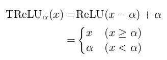
      * `alpha` is a learned parameter.
      * TReLUs play better with their WN layers than normal ReLUs.
  * Reconstruction measure
    * To evaluate the quality of the generated images during training, they introduce a new measure.
    * The measure is based on a L2-Norm (MSE) between (1) a real image and (2) an image created by the generator that is as similar as possible to the real image.
    * They generate (2) by starting `G(z)` with a noise vector `z` that is filled with zeros. The desired output is the real image. They compute a MSE between the generated and real image and backpropagate the result. Then they use the generated gradient to update `z`, while leaving the parameters of `G` unaltered. They repeat this for a defined number of steps.
    * Note that the above described method is fairly time-consuming, so they don't do it often.
  * Networks
    * Their networks are fairly standard.
    * Generator: Starts at 1024 filters, goes down to 64 (then 3 for the output). Upsampling via fractionally strided convs.
    * Discriminator: Starts at 64 filters, goes to 1024 (then 1 for the output). Downsampling via strided convolutions.
    * They test three variations of these networks:
      * Vanilla: No normalization. PReLUs in both G and D.
      * BN: BN in G and D, but not in the last layers and not in the first layer of D. PReLUs in both G and D.
      * WN: Strict weight-normalized layers in G and D, except for the last layers, which are affine weight-normalized layers. TPReLUs (Translated PReLUs) in both G and D.
  * Other
    * They train with RMSProp and batch size 32.

### Results
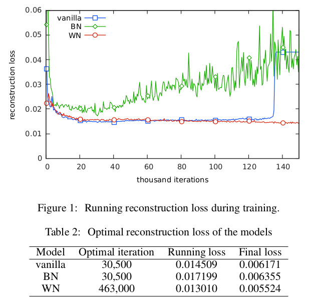
  * Their WN formulation trains stable, provided the learning rate is set to 0.0002 or lower.
  * They argue, that their achieved stability is similar to the one in WGAN.
  * BN had significant swings in quality.
  * Vanilla collapsed sooner or later.
  * Both BN and Vanilla reached an optimal point shortly after the start of the training. After that, the quality of the generated images only worsened.
  * Plot of their quality measure:
    * ![Losses over time](https://raw.githubusercontent.com/aleju/papers/master/neural-nets/images/On_the_Effects_of_BN_and_WN_in_GANs__losses_over_time.jpg?raw=true "Losses over time")
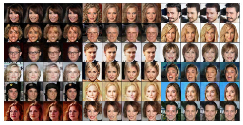
  * Their quality measure is based on reconstruction of input images. The below image shows examples for that reconstruction (each person: original image, vanilla reconstruction, BN rec., WN rec.).
    * ![Reconstructions](https://raw.githubusercontent.com/aleju/papers/master/neural-nets/images/On_the_Effects_of_BN_and_WN_in_GANs__reconstructions.jpg?raw=true "Reconstructions")
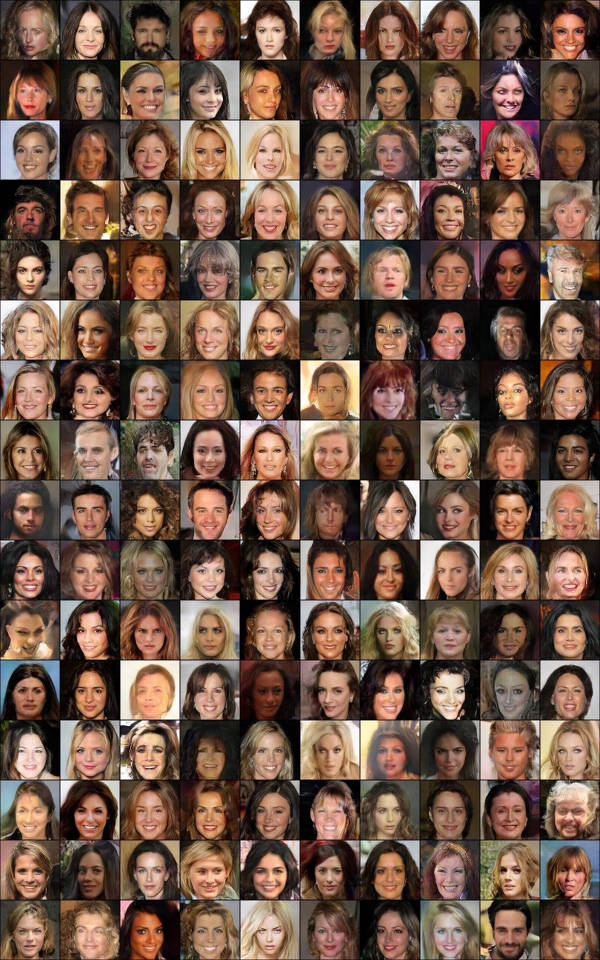
  * Examples generated by their WN network:
    * ![WN Examples](https://raw.githubusercontent.com/aleju/papers/master/neural-nets/images/On_the_Effects_of_BN_and_WN_in_GANs__wn_examples.jpg?raw=true "WN Examples")