#### Motivation:

+ Take advantage of the fact that missing values can be very informative about the label.
+ Sampling a time series generates many missing values.

![Sampling](https://raw.githubusercontent.com/tiagotvv/ml-papers/master/clinical-data/images/Lipton2016_motivation.png?raw=true)


#### Model (indicator flag):

+ Indicator of occurrence of missing value.

![Indicator](https://raw.githubusercontent.com/tiagotvv/ml-papers/master/clinical-data/images/Lipton2016_indicator.png?raw=true)

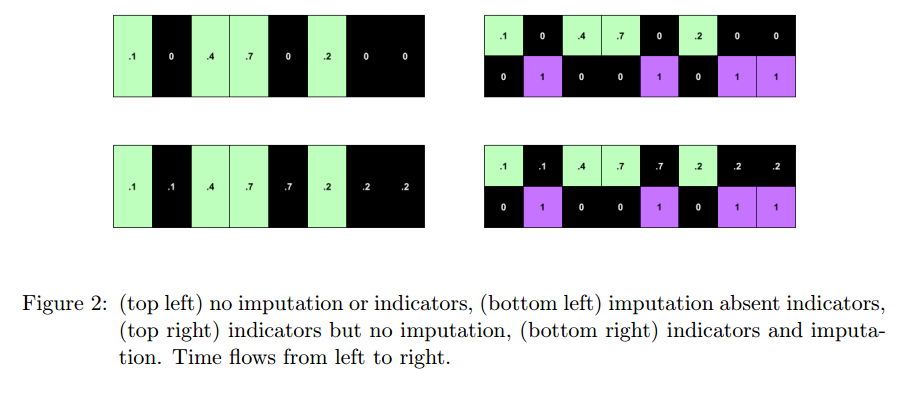
+ An RNN can learn about missing values and their importance only by using the indicator function. The nonlinearity from this type of model helps capturing these dependencies.
+ If one wants to use a linear model, feature engineering is needed to overcome its limitations.
  + indicator for whether a variable was measured at all
  + mean and standard deviation of the indicator 
  + frequency with which a variable switches from measured to missing and vice-versa. 

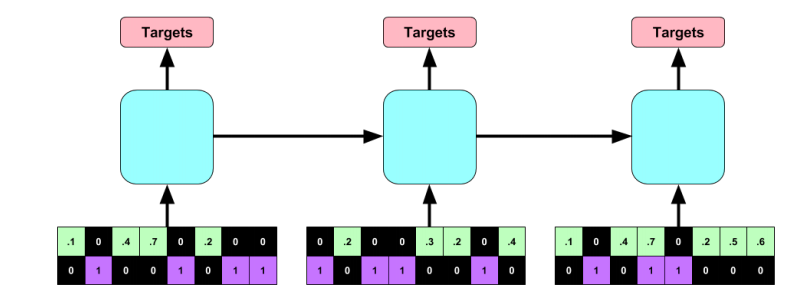
#### Architecture:

+ RNN with target replication following the work "Learning to Diagnose with LSTM Recurrent Neural Networks" by the same authors.

![Architecture](https://raw.githubusercontent.com/tiagotvv/ml-papers/master/clinical-data/images/Lipton2016_architecture.png?raw=true)


#### Dataset:

+ Children's Hospital LA
+ Episode is a multivariate time series that describes the stay of one patient in the intensive care unit

Dataset properties  | Value 
---------|----------
Number of episodes | 10,401
Duration of episodes | From 12h to several months
Time series variables | Systolic blood pressure, Diastolic blood pressure,  Peripheral capillary refill rate, End tidal CO2, Fraction of inspired O2,  Glasgow coma scale,  Blood glucose,  Heart rate,  pH,  Respiratory rate, Blood O2 Saturation,  Body temperature,  Urine output.



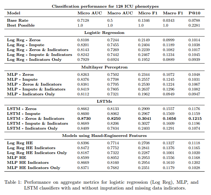
#### Experiments and Results:

**Goal**
+ Predict 128 diagnoses.
+ Multilabel: patients can have more than one diagnose.

**Methodology**
+ Split: 80% training, 10% validation, 10% test.
+ Normalized data to be in the range [0,1].

+ LSTM RNN:
  + 2 hidden layers with 128 cells. Dropout = 0.5, L2-regularization: 1e-6
  + Training for 100 epochs. Parameters chosen correspond to the time that generated the smallest error in the validation dataset.
+ Baselines:
  + Logistic Regression (L2 regularization)
  + MLP with 3 hidden layers and 500 hidden neurons / layer (parameters chosen via validation set)
  + Tested with raw-features and hand-engineered features.
+ Strategies for missing values:
  + Zeroing
  + Impute via forward / backfilling
  + Impute with zeros and use indicator function
  + Impute via forward / backfilling and use indicator function
  + Use indicator function only

#### Results

+ Metrics:
  + Micro AUC, Micro F1: calculated by adding the TPs, FPs, TNs and FNs for the entire dataset and for all classes.
  + Macro AUC, Macro F1: Arithmetic mean of AUCs and F1 scores for each of the classes.
  + Precision at 10: Fraction of correct diagnostics among the top 10 predictions of the model.
    + The upper bound for precision at 10 is 0.2281 since in the test set there are on average 2.281 diagnoses per patient.

![Results](https://raw.githubusercontent.com/tiagotvv/ml-papers/master/clinical-data/images/Lipton2016_results.png?raw=true)


#### Discussion:

+ Predictive model based on data collected following a given routine. This routine can change if the model is put into practice. Will the model predictions in this new routine remain valid?

+ Missing values in a way give an indication of the type of treatment being followed.

+ Trade-off between complex models operating on raw features and very complex features operating on more interpretable models.

  * They suggest a factorization of standard 3x3 convolutions that is more efficient.
  * They build a model based on that factorization. The model has hyperparameters to choose higher performance or higher accuracy.

### How
  * Factorization
    * They factorize the standard 3x3 convolution into one depthwise 3x3 convolution, followed by a pointwise convoluton.
    * Normal 3x3 convolution:
      * Computes per filter and location a weighted average over all filters.
      * For kernel height `kH`, width `kW` and number of input filters/planes `Fin`, it requires `kH*kW*Fin` computations per location.
    * Depthwise 3x3 convolution:
      * Computes per filter and location a weighted average over *one* input filter. E.g. the 13th filter would only computed weighted averages over the 13th input filter/plane and ignore all the other input filters/planes.
      * This requires `kH*kW*1` computations per location, i.e. drastically less than a normal convolution.
    * Pointwise convolution:
      * This is just another name for a normal 1x1 convolution.
      * This is placed after a depthwise convolution in order to compensate the fact that every (depthwise) filter only sees a single input plane.
      * As the kernel size is `1`, this is rather fast to compute.
    * Visualization of normal vs factorized convolution:
      * ![architecture](https://github.com/aleju/papers/blob/master/neural-nets/images/MobileNets/architecture.jpg?raw=true "architecture")
  * Models
    * They use two hyperparameters for their models.
    * `alpha`: Multiplier for the width in the range `(0, 1]`. A value of 0.5 means that every layer has half as many filters.
    * `roh`: Multiplier for the resolution. In practice this is simply the input image size, having a value of `{224, 192, 160, 128}`.

### Results
  * ImageNet
    * Compared to VGG16, they achieve 1 percentage point less accuracy, while using only about 4% of VGG's multiply and additions (mult-adds) and while using only about 3% of the parameters.
    * Compared to GoogleNet, they achieve about 1 percentage point more accuracy, while using only about 36% of the mult-adds and 61% of the parameters.
    * Note that they don't compare to ResNet.
    * Results for architecture choices vs. accuracy on ImageNet:
      * ![results imagenet](https://github.com/aleju/papers/blob/master/neural-nets/images/MobileNets/results_imagenet.jpg?raw=true "results imagenet")
    * Relation between mult-adds and accuracy on ImageNet:
      * ![mult-adds vs accuracy](https://github.com/aleju/papers/blob/master/neural-nets/images/MobileNets/mult-adds_vs_accuracy.jpg?raw=true "mult-adds vs accuracy")
  * Object Detection
    * Their mAP is a bit on COCO when combining MobileNet with SSD (as opposed to using VGG or Inception v2).
    * Their mAP is quite a bit worse on COCO when combining MobileNet with Faster R-CNN.
  * Reducing the number of filters (`alpha`) influences the results more than reducing the input image resolution (`roh`).
  * Making the models shallower influences the results more than making them thinner.

  * They suggest a modified network architecture for object detectors (i.e. bounding box detectors).
  * The architecture aggregates features from many scales (i.e. before each pooling layer) to detect both small and large object.
  * The network is shaped similar to an hourglass.

###  How
  * Architecture
    * They have two branches.
    * The first one is similar to any normal network:
      Convolutions and pooling.
      The exact choice of convolutions (e.g. how many) and pooling is determined by the used base network (e.g. ~50 convolutions with ~5x pooling in ResNet-50).
    * The second branch starts at the first one's output.
      It uses nearest neighbour upsampling to re-increase the resolution back to the original one.
      It does not contain convolutions.
      All layers have 256 channels.
    * There are connections between the layers of the first and second branch.
      These connections are simply 1x1 convolutions followed by an addition (similar to residual connections).
      Only layers with similar height and width are connected.
    * Visualization:
      * ![architecture](https://github.com/aleju/papers/blob/master/neural-nets/images/Feature_Pyramid_Networks_for_Object_Detection/architecture.jpg?raw=true "architecture")
  * Integration with Faster R-CNN
    * They base the RPN on their second branch.
    * While usually an RPN is applied to a single feature map of one scale, in their case it is applied to many feature maps of varying scales.
    * The RPN uses the same parameters for all scales.
    * They use anchor boxes, but only of different aspect ratios, not of different scales (as scales are already covered by their feature map heights/widths).
    * Ground truth bounding boxes are associated with the best matching anchor box (i.e. one box among all scales).
    * Everything else is the same as in Faster R-CNN.
  * Integration with Fast R-CNN
    * Fast R-CNN does not use an RPN, but instead usually uses Selective Search to find region proposals (and applies RoI-Pooling to them).
    * Here, they simply RoI-Pool from the FPN's output of the second branch.
    * They do not pool over all scales. Instead they pick only the scale/layer that matches the region proposal's size (based on its height/width).
    * They process each pooled RoI using two 1024-dimensional fully connected layers (initalizes randomly).
    * Everything else is the same as in Fast R-CNN.

### Results
  * Faster R-CNN
    * FPN improves recall on COCO by about 8 points, compared to using standard RPN.
    * Improvement is stronger for small objects (about 12 points).
    * For some reason no AP values here, only recall.
    * The RPN uses some convolutions to transform each feature map into region proposals.
      Sharing the features of these convolutions marginally improves results.
  * Fast R-CNN
    * FPN improves AP on COCO by about 2 points.
    * Improvement is stronger for small objects (about 2.1 points).

  * Deep plain/ordinary networks usually perform better than shallow networks.
  * However, when they get too deep their performance on the *training* set decreases. That should never happen and is a shortcoming of current optimizers.
  * If the "good" insights of the early layers could be transferred through the network unaltered, while changing/improving the "bad" insights, that effect might disappear.

###  What residual architectures are
  * Residual architectures use identity functions to transfer results from previous layers unaltered.
  * They change these previous results based on results from convolutional layers.
  * So while a plain network might do something like `output = convolution(image)`, a residual network will do `output = image + convolution(image)`.
  * If the convolution resorts to just doing nothing, that will make the result a lot worse in the plain network, but not alter it at all in the residual network.
  * So in the residual network, the convolution can focus fully on learning what positive changes it has to perform, while in the plain network it *first* has to learn the identity function and then what positive changes it can perform.

### How it works
  * Residual architectures can be implemented in most frameworks. You only need something like a split layer and an element-wise addition.
  * Use one branch with an identity function and one with 2 or more convolutions (1 is also possible, but seems to perform poorly). Merge them with the element-wise addition.
  * Rough example block (for a 64x32x32 input):
https://i.imgur.com/NJVb9hj.png  
  * An example block when you have to change the dimensionality (e.g. here from 64x32x32 to 128x32x32):
https://i.imgur.com/9NXvTjI.png
  * The authors seem to prefer using either two 3x3 convolutions or the chain of 1x1 then 3x3 then 1x1. They use the latter one for their very deep networks.
  * The authors also tested:
    * To use 1x1 convolutions instead of identity functions everywhere. Performed a bit better than using 1x1 only for dimensionality changes. However, also computation and memory demands.
    * To use zero-padding for dimensionality changes (no 1x1 convs, just fill the additional dimensions with zeros). Performed only a bit worse than 1x1 convs and a lot better than plain network architectures.
  * Pooling can be used as in plain networks. No special architectures are necessary.
  * Batch normalization can be used as usually (before nonlinearities).

### Results
  * Residual networks seem to perform generally better than similarly sized plain networks.
  * They seem to be able to achieve similar results with less computation.
  * They enable well-trainable very deep architectures with up to 1000 layers and more.
  * The activations of the residual layers are low compared to plain networks. That indicates that the residual networks indeed only learn to make "good" changes and default to "if in doubt, change nothing".


![Building blocks](https://raw.githubusercontent.com/aleju/papers/master/neural-nets/images/Deep_Residual_Learning_for_Image_Recognition__building_blocks.png?raw=true "Building blocks")

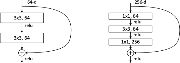
*Examples of basic building blocks (other architectures are possible). The paper doesn't discuss the placement of the ReLU (after add instead of after the layer).*


![Activations](https://raw.githubusercontent.com/aleju/papers/master/neural-nets/images/Deep_Residual_Learning_for_Image_Recognition__activations.png?raw=true "Activations")

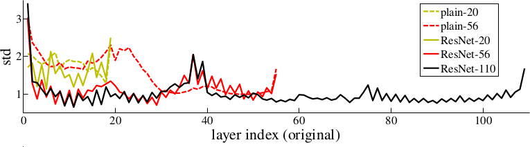
*Activations of layers (after batch normalization, before nonlinearity) throughout the network for plain and residual nets. Residual networks have on average lower activations.*

-------------------------

### Rough chapter-wise notes

* (1) Introduction
  * In classical architectures, adding more layers can cause the network to perform worse on the training set.
  * That shouldn't be the case. (E.g. a shallower could be trained and then get a few layers of identity functions on top of it to create a deep network.)
  * To combat that problem, they stack residual layers.
  * A residual layer is an identity function and can learn to add something on top of that.
  * So if `x` is an input image and `f(x)` is a convolution, they do something like `x + f(x)` or even `x + f(f(x))`.
  * The classical architecture would be more like `f(f(f(f(x))))`.
  * Residual architectures can be easily implemented in existing frameworks using skip connections with identity functions (split + merge).
  * Residual architecture outperformed other in ILSVRC 2015 and COCO 2015.

* (3) Deep Residual Learning
  * If some layers have to fit a function `H(x)` then they should also be able to fit `H(x) - x` (change between `x` and `H(x)`).
  * The latter case might be easier to learn than the former one.
  * The basic structure of a residual block is `y = x + F(x, W)`, where `x` is the input image, `y` is the output image (`x + change`) and `F(x, W)` is the residual subnetwork that estimates a good change of `x` (W are the subnetwork's weights).
  * `x` and `F(x, W)` are added using element-wise addition.
  * `x` and the output of `F(x, W)` must be have equal dimensions (channels, height, width).
  * If different dimensions are required (mainly change in number of channels) a linear projection `V` is applied to `x`: `y = F(x, W) + Vx`. They use a 1x1 convolution for `V` (without nonlinearity?).
  * `F(x, W)` subnetworks can contain any number of layer. They suggest 2+ convolutions. Using only 1 layer seems to be useless.
  * They run some tests on a network with 34 layers and compare to a 34 layer network without residual blocks and with VGG (19 layers).
  * They say that their architecture requires only 18% of the FLOPs of VGG. (Though a lot of that probably comes from VGG's 2x4096 fully connected layers? They don't use any fully connected layers, only convolutions.)
  * A critical part is the change in dimensionality (e.g. from 64 kernels to 128). They test (A) adding the new dimensions empty (padding), (B) using the mentioned linear projection with 1x1 convolutions and (C) using the same linear projection, but on all residual blocks (not only for dimensionality changes).
  * (A) doesn't add parameters, (B) does (i.e. breaks the pattern of using identity functions).
  * They use batch normalization before each nonlinearity.
  * Optimizer is SGD.
  * They don't use dropout.

* (4) Experiments
  * When testing on ImageNet an 18 layer plain (i.e. not residual) network has lower training set error than a deep 34 layer plain network.
  * They argue that this effect does probably not come from vanishing gradients, because they (a) checked the gradient norms and they looked healthy and (b) use batch normaliaztion.
  * They guess that deep plain networks might have exponentially low convergence rates.
  * For the residual architectures its the other way round. Stacking more layers improves the results.
  * The residual networks also perform better (in error %) than plain networks with the same number of parameters and layers. (Both for training and validation set.)
  * Regarding the previously mentioned handling of dimensionality changes:
    * (A) Pad new dimensions: Performs worst. (Still far better than plain network though.)
    * (B) Linear projections for dimensionality changes: Performs better than A.
    * (C) Linear projections for all residual blocks: Performs better than B. (Authors think that's due to introducing new parameters.)
  * They also test on very deep residual networks with 50 to 152 layers.
  * For these deep networks their residual block has the form `1x1 conv -> 3x3 conv -> 1x1 conv` (i.e. dimensionality reduction, convolution, dimensionality increase).
  * These deeper networks perform significantly better.
  * In further tests on CIFAR-10 they can observe that the activations of the convolutions in residual networks are lower than in plain networks.
  * So the residual networks default to doing nothing and only change (activate) when something needs to be changed.
  * They test a network with 1202 layers. It is still easily optimizable, but overfits the training set.
  * They also test on COCO and get significantly better results than a Faster-R-CNN+VGG implementation.

  * ELUs are an activation function
  * The are most similar to LeakyReLUs and PReLUs

### How (formula)
  * f(x):
    * `if x >= 0: x`
    * `else: alpha(exp(x)-1)`
  * f'(x) / Derivative:
    * `if x >= 0: 1`
    * `else: f(x) + alpha`
  * `alpha` defines at which negative value the ELU saturates.
  * E. g. `alpha=1.0` means that the minimum value that the ELU can reach is `-1.0`
  * LeakyReLUs however can go to `-Infinity`, ReLUs can't go below 0.

![ELUs vs LeakyReLUs vs ReLUs](https://raw.githubusercontent.com/aleju/papers/master/neural-nets/images/ELUs__slopes.png?raw=true "ELUs vs LeakyReLUs vs ReLUs")

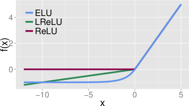
*Form of ELUs(alpha=1.0) vs LeakyReLUs vs ReLUs.*


### Why
  * They derive from the unit natural gradient that a network learns faster, if the mean activation of each neuron is close to zero.
  * ReLUs can go above 0, but never below. So their mean activation will usually be quite a bit above 0, which should slow down learning.
  * ELUs, LeakyReLUs and PReLUs all have negative slopes, so their mean activations should be closer to 0.
  * In contrast to LeakyReLUs and PReLUs, ELUs saturate at a negative value (usually -1.0).
  * The authors think that is good, because it lets ELUs encode the degree of presence of input concepts, while they do not quantify the degree of absence.
  * So ELUs can measure the presence of concepts quantitatively, but the absence only qualitatively.
  * They think that this makes ELUs more robust to noise.

### Results
  * In their tests on MNIST, CIFAR-10, CIFAR-100 and ImageNet, ELUs perform (nearly always) better than ReLUs and LeakyReLUs.
  * However, they don't test PReLUs at all and use an alpha of 0.1 for LeakyReLUs (even though 0.33 is afaik standard) and don't test LeakyReLUs on ImageNet (only ReLUs).

![CIFAR-100](https://raw.githubusercontent.com/aleju/papers/master/neural-nets/images/ELUs__cifar100.png?raw=true "CIFAR-100")

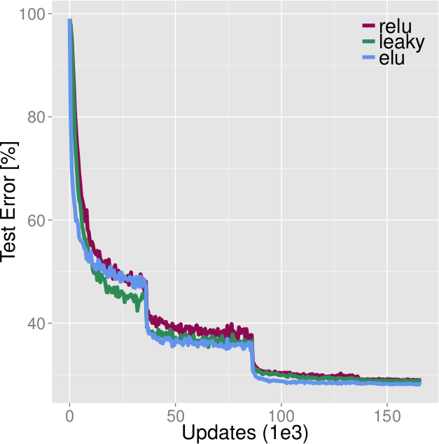
*Comparison of ELUs, LeakyReLUs, ReLUs on CIFAR-100. ELUs ends up with best values, beaten during the early epochs by LeakyReLUs. (Learning rates were optimized for ReLUs.)*

-------------------------

### Rough chapter-wise notes

* Introduction
  * Currently popular choice: ReLUs
  * ReLU: max(0, x)
  * ReLUs are sparse and avoid the vanishing gradient problem, because their derivate is 1 when they are active.
  * ReLUs have a mean activation larger than zero.
  * Non-zero mean activation causes a bias shift in the next layer, especially if multiple of them are correlated.
  * The natural gradient (?) corrects for the bias shift by adjusting the weight update.
  * Having less bias shift would bring the standard gradient closer to the natural gradient, which would lead to faster learning.
  * Suggested solutions:
    * Centering activation functions at zero, which would keep the off-diagonal entries of the Fisher information matrix small.
    * Batch Normalization
    * Projected Natural Gradient Descent (implicitly whitens the activations)
  * These solutions have the problem, that they might end up taking away previous learning steps, which would slow down learning unnecessarily.
  * Chosing a good activation function would be a better solution.
  * Previously, tanh was prefered over sigmoid for that reason (pushed mean towards zero).
  * Recent new activation functions:
    * LeakyReLUs: x if x > 0, else alpha*x
    * PReLUs: Like LeakyReLUs, but alpha is learned
    * RReLUs: Slope of part < 0 is sampled randomly
  * Such activation functions with non-zero slopes for negative values seemed to improve results.
  * The deactivation state of such units is not very robust to noise, can get very negative.
  * They suggest an activation function that can return negative values, but quickly saturates (for negative values, not for positive ones).
  * So the model can make a quantitative assessment for positive statements (there is an amount X of A in the image), but only a qualitative negative one (something indicates that B is not in the image).
  * They argue that this makes their activation function more robust to noise.
  * Their activation function still has activations with a mean close to zero.

* Zero Mean Activations Speed Up Learning
  * Natural Gradient = Update direction which corrects the gradient direction with the Fisher Information Matrix
  * Hessian-Free Optimization techniques use an extended Gauss-Newton approximation of Hessians and therefore can be interpreted as versions of natural gradient descent.
  * Computing the Fisher matrix is too expensive for neural networks.
  * Methods to approximate the Fisher matrix or to perform natural gradient descent have been developed.
  * Natural gradient = inverse(FisherMatrix) * gradientOfWeights
  * Lots of formulas. Apparently first explaining how the natural gradient descent works, then proofing that natural gradient descent can deal well with non-zero-mean activations.
  * Natural gradient descent auto-corrects bias shift (i.e. non-zero-mean activations).
  * If that auto-correction does not exist, oscillations (?) can occur, which slow down learning.
  * Two ways to push means towards zero:
    * Unit zero mean normalization (e.g. Batch Normalization)
    * Activation functions with negative parts

* Exponential Linear Units (ELUs)
  * *Formula*
    * f(x):
      * if x >= 0: x
      * else: alpha(exp(x)-1)
    * f'(x) / Derivative:
      * if x >= 0: 1
      * else: f(x) + alpha
    * `alpha` defines at which negative value the ELU saturates.
    * `alpha=0.5` => minimum value is -0.5 (?)
  * ELUs avoid the vanishing gradient problem, because their positive part is the identity function (like e.g. ReLUs)
  * The negative values of ELUs push the mean activation towards zero.
  * Mean activations closer to zero resemble more the natural gradient, therefore they should speed up learning.
  * ELUs are more noise robust than PReLUs and LeakyReLUs, because their negative values saturate and thus should create a small gradient.
  * "ELUs encode the degree of presence of input concepts, while they do not quantify the degree of absence"

* Experiments Using ELUs
  * They compare ELUs to ReLUs and LeakyReLUs, but not to PReLUs (no explanation why).
  * They seem to use a negative slope of 0.1 for LeakyReLUs, even though 0.33 is standard afaik.
  * They use an alpha of 1.0 for their ELUs (i.e. minimum value is -1.0).
  * MNIST classification:
    * ELUs achieved lower mean activations than ReLU/LeakyReLU
    * ELUs achieved lower cross entropy loss than ReLU/LeakyReLU (and also seemed to learn faster)
    * They used 5 hidden layers of 256 units each (no explanation why so many)
    * (No convolutions)
  * MNIST Autoencoder:
    * ELUs performed consistently best (at different learning rates)
    * Usually ELU > LeakyReLU > ReLU
    * LeakyReLUs not far off, so if they had used a 0.33 value maybe these would have won
  * CIFAR-100 classification:
    * Convolutional network, 11 conv layers
    * LeakyReLUs performed better during the first ~50 epochs, ReLUs mostly on par with ELUs
    * LeakyReLUs about on par for epochs 50-100
    * ELUs win in the end (the learning rates used might not be optimal for ELUs, were designed for ReLUs)
  * CIFER-100, CIFAR-10 (big convnet):
    * 6.55% error on CIFAR-10, 24.28% on CIFAR-100
    * No comparison with ReLUs and LeakyReLUs for same architecture
  * ImageNet
    * Big convnet with spatial pyramid pooling (?) before the fully connected layers
    * Network with ELUs performed better than ReLU network (better score at end, faster learning)
    * Networks were still learning at the end, they didn't run till convergence
    * No comparison to LeakyReLUs