In this work they take a different approach to the GAN model \cite{1406.2661}. In the traditionally GAN model a neural network is trained to up-sample from random noise in a feed forward fashion to generate samples from the data distribution. 

This work instead iteratively permutes an image of random noise similar to Artistic Style Transfer \cite{1508.06576}.  The image is permuted in order to fool a set of discriminators. To obtain the set of discriminators each is trained starting from random noise until some max $t$ step. 


1. At first a discriminator is trained to discriminate between the true data and random noise . 
2. Images is then permuted using gradients which aim to fool the discriminator and included in the data distribution as a negative example.
3. The discriminator is trained on the true data + random noise + fake data from the previous steps

The images generated at each step are shown below:

https://i.imgur.com/kp575s8.png

After being trained the model is able to generate a sample by iterating over each trained discriminator and applying gradient updates on from random noise. For this storing only the weights of the discriminators is required.

Poster from ICCV2017:
https://i.imgur.com/vYSSdZx.png

This work deals with rotation equivariant convolutional filters. The idea is that when you rotate an image you should not need to relearn new filters to deal with this rotation. First we can look at how convolutions typically handle rotation and how we would expect a rotation invariant solution to perform below:

| | |
| - | - |
| https://i.imgur.com/cirTi4S.png | https://i.imgur.com/iGpUZDC.png |
| | | |

The method computes all possible rotations of the filter which results in a list of activations where each element represents a different rotation. From this list the maximum is taken which results in a two dimensional output for every pixel (rotation, magnitude). This happens at the pixel level so the result is a vector field over the image.


https://i.imgur.com/BcnuI1d.png

We can visualize their degree selection method with a figure from https://arxiv.org/abs/1603.04392 which determined the rotation of a building:

https://i.imgur.com/hPI8J6y.png

We can also think of this approach as attention \cite{1409.0473} where they attend over the possible rotations to obtain a score for each possible rotation value to pass on. The network can learn to adjust the rotation value to be whatever value the later layers will need. 

------------------------

Results on [Rotated MNIST](http://www.iro.umontreal.ca/~lisa/twiki/bin/view.cgi/Public/MnistVariations) show an impressive improvement in training speed and generalization error:




https://i.imgur.com/YO3poOO.png

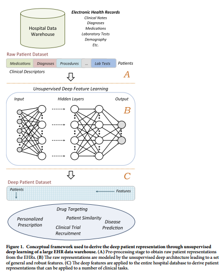
#### Goal

+ Use unsupervised deep learning to obtain a low-dimensional representation of a patient from EHR data. 
+ A better representation will facilitate clinical prediction tasks.

#### Architecture:

+ Patient EHR is obtained from the Hospital Data Warehouse:
  + demographic info 
  + ICD-9 codes 
  + medication, labs
  + clinical notes: free text 
+ Use stacked denoising autoencoders (SDA) to obtain an abstract representation of the patient with lower dimensionality.

![Framework](https://raw.githubusercontent.com/tiagotvv/ml-papers/master/clinical-data/images/Miotto2016_framework.png?raw=true "Deep Patient Framework")

#### Dataset:

+ Data Warehouse from Mount Sinai Hospital in NY.
+ All patient records that had a diagnosed disease (ICD-9 code) between 1980 and 2014 - approximately 1.2 million patients with 88.9 records/patient - were initially selected.
  + 1980-2013: training, 2014: test.

*Data Cleaning*:
+ Diseases diagnosed in fewer than 10 patients in the training dataset were eliminated.
+ Diseases that could not be diagnosed through EHR labels were eliminated. Related to social behavior (HIV), fortuitous events (injuries, poisoning) or unspecific ('other cancers'). The final list contains 78 diseases.

*Final version of the dataset (raw patient representation)*:

+ Training: 704,587 patients (to obtain deep features post SDA).
+ Validation: 5,000 patients (for the evaluation of the predictive model for diseases).
+ Test: 76,214 patients (for the evaluation of the predictive model for diseases).
+ 41072 columns - demographic info, ICD-9, medication, lab test, free text (LDA topic modeling dimension 300)
+ Very high dimensional but very sparse representation

#### Results:

*Stacked Denoisinig Autoencoders for low-dimensional patient representation*:
+ 3 layers of denoising autoencoders.
+ Each layer has 500 neurons. Patient is now represented by a dense vector of 500 features.
+ Inputs are normalized to lie in the [0, 1] interval.
+ Inputs in each of the layers have added noise at a ratio of 5% noise (masking noise corruption - value of these features is set to '0').
+ Sigmoid activation function.

*Classifiers for disease prediction*:
+ Random forest classifiers with 100 trees trained for each of the 78 diseases.

*Baseline for comparison*:
+ PCA with 100 components, k-means with 500 clusters, GMM with 200 mixes and ICA with 100 components. (see Discussion)
+ RawFeat: original patient EHR features: sparse vector with 41072 features (~ 1% of non-zero entries).
+ Threshold to rank as "positive": 0.6

*Aggregate performance in predicting diseases*:

![Aggregate performance](https://raw.githubusercontent.com/tiagotvv/ml-papers/master/clinical-data/images/Miotto2016_results1.png?raw=true "Aggregate performance")

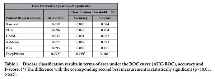
+ Comment: This result of F-Score = 0.181 implies a precision of 0.102 (let us assume a recall in the order of 80%), which means that with each correct diagnosis, the Deep Patient generates approximately 9 false alarms.

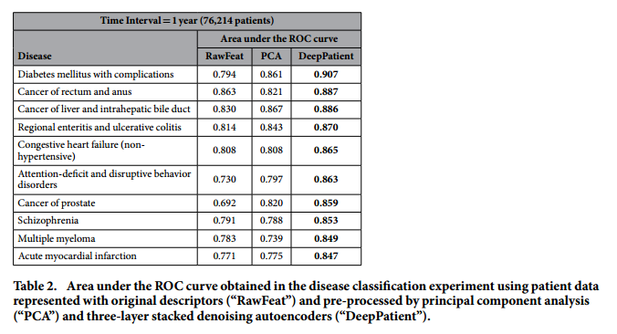
*Performance for some particular diseases*:

![Disease results](https://raw.githubusercontent.com/tiagotvv/ml-papers/master/clinical-data/images/Miotto2016_results2.png?raw=true "Results for some diseases")

#### Discussion:
+ DeepPatient *does not* use lab results in model building. Only the *frequency* at which the analysis is performed is taken into account.
+ Future enhancements:
  +  Describe a patient with a temporal sequence of vectors s instead of summarizing all data in one vector.
  +  Add other categories of EHR data, such as insurance details, family history and social behaviors.
  + Use PCA as a pre-processing step before SDA?
+ Caveat: the comparisons does not seem to be fair. If the autoencoder has dimension 500, the other baselines should also have dimension 500. 

  * The original GAN approach used one Generator (G) to generate images and one Discriminator (D) to rate these images.
  * The laplacian pyramid GAN uses multiple pairs of G and D.
  * It starts with an ordinary GAN that generates small images (say, 4x4).
  * Each following pair learns to generate plausible upscalings of the image, usually by a factor of 2. (So e.g. from 4x4 to 8x8.)
  * This scaling from coarse to fine resembles a laplacian pyramid, hence the name.

### How
  * The first pair of G and D is just like an ordinary GAN.
  * For each pair afterwards, G recieves the output of the previous step, upscaled to the desired size. Due to the upscaling, the image will be blurry.
  * G has to learn to generate a plausible sharpening of that blurry image.
  * G outputs a difference image, not the full sharpened image.
  * D recieves the upscaled/blurry image. D also recieves either the optimal difference image (for images from the training set) or G's generated difference image.
  * D adds the difference image to the blurry image as its first step. Afterwards it applies convolutions to the image and ends in one sigmoid unit.
  * The training procedure is just like in the ordinary GAN setting. Each upscaling pair of G and D can be trained on its own.
  * The first G recieves a "normal" noise vector, just like in the ordinary GAN setting. Later Gs recieve noise as one plane, so each image has four channels: R, G, B, noise.

### Results
  * Images are rated as looking more realistic than the ones from ordinary GANs.
  * The approximated log likelihood is significantly lower (improved) compared to ordinary GANs.
  * The generated images do however still look distorted compared to real images.
  * They also tried to add class conditional information to G and D (just a one hot vector for the desired class of the image). G and D learned successfully to adapt to that information (e.g. to only generate images that seem to show birds).



![Sampling Process](https://raw.githubusercontent.com/aleju/papers/master/neural-nets/images/Deep_Generative_Image_Models_using_a_Laplacian_Pyramid_of_Adversarial_Networks__pyramid.png?raw=true "Sampling process")

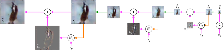
*Basic training and sampling process. The first image is generated directly from noise. Everything afterwards is de-blurring of upscaled images.*


-------------------------

### Rough chapter-wise notes

* Introduction
  * Instead of just one big generative model, they build multiple ones.
  * They start with one model at a small image scale (e.g. 4x4) and then add multiple generative models that increase the image size (e.g. from 4x4 to 8x8).
  * This scaling from coarse to fine (low frequency to high frequency components) resembles a laplacian pyramid, hence the name of the paper.

* Related Works
  * Types of generative image models:
    * Non-Parametric: Models copy patches from training set (e.g. texture synthesis, super-resolution)
    * Parametric: E.g. Deep Boltzmann machines or denoising auto-encoders
  * Novel approaches: e.g. DRAW, diffusion-based processes, LSTMs
  * This work is based on (conditional) GANs

* Approach
  * They start with a Gaussian and a Laplacian pyramid.
  * They build the Gaussian pyramid by repeatedly decreasing the image height/width by 2: [full size image, half size image, quarter size image, ...]
  * They build a Laplacian pyramid by taking pairs of images in the gaussian pyramid, upscaling the smaller one and then taking the difference.
  * In the laplacian GAN approach, an image at scale k is created by first upscaling the image at scale k-1 and then adding a refinement to it (de-blurring). The refinement is created with a GAN that recieves the upscaled image as input.
  * Note that the refinement is a difference image (between the upscaled image and the optimal upscaled image).
  * The very first (small scale) image is generated by an ordinary GAN.
  * D recieves an upscaled image and a difference image. It then adds them together to create an upscaled and de-blurred image. Then D applies ordinary convolutions to the result and ends in a quality rating (sigmoid).

* Model Architecture and Training
  * Datasets: CIFAR-10 (32x32, 100k images), STL (96x96, 100k), LSUN (64x64, 10M)
  * They use a uniform distribution of [-1, 1] for their noise vectors.
  * For the upscaling Generators they add the noise as a fourth plane (to the RGB image).
  * CIFAR-10: 8->14->28 (height/width), STL: 8->16->32->64->96, LSUN: 4->8->16->32->64
  * CIFAR-10: G=3 layers, D=2 layers, STL: G=3 layers, D=2 layers, LSUN: G=5 layers, D=3 layers.

* Experiments
  * Evaluation methods:
    * Computation of log-likelihood on a held out image set
      * They use a Gaussian window based Parzen estimation to approximate the probability of an image (note: not very accurate).
      * They adapt their estimation method to the special case of the laplacian pyramid.
      * Their laplacian pyramid model seems to perform significantly better than ordinary GANs.
    * Subjective evaluation of generated images
      * Their model seems to learn the rough structure and color correlations of images to generate.
      * They add class conditional information to G and D. G indeed learns to generate different classes of images.
      * All images still have noticeable distortions.
    * Subjective evaluation of generated images by other people
      * 15 volunteers.
      * They show generated or real images in an interface for 50-2000ms. Volunteer then has to decide whether the image is fake or real.
      * 10k ratings were collected.
      * At 2000ms, around 50% of the generated images were considered real, ~90 of the true real ones and <10% of the images generated by an ordinary GAN. 

  * DRAW = deep recurrent attentive writer
  * DRAW is a recurrent autoencoder for (primarily) images that uses attention mechanisms.
  * Like all autoencoders it has an encoder, a latent layer `Z` in the "middle" and a decoder.
  * Due to the recurrence, there are actually multiple autoencoders, one for each timestep (the number of timesteps is fixed).
  * DRAW has attention mechanisms which allow the model to decide where to look at in the input image ("glimpses") and where to write/draw to in the output image.
  * If the attention mechanisms are skipped, the model becomes a simple recurrent autoencoder.
  * By training the full autoencoder on a dataset and then only using the decoder, one can generate new images that look similar to the dataset images.


![DRAW Architecture](https://raw.githubusercontent.com/aleju/papers/master/neural-nets/images/DRAW_A_Recurrent_Neural_Network_for_Image_Generation__architecture.png?raw=true "DRAW Architecture")

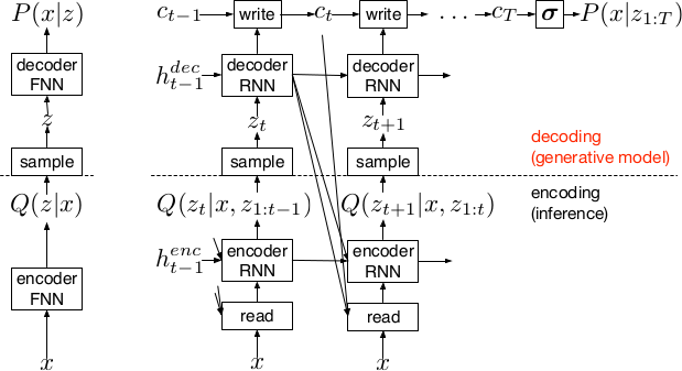
*Basic recurrent architecture of DRAW.*


### How
  * General architecture
    * The encoder-decoder-pair follows the design of variational autoencoders.
    * The latent layer follows an n-dimensional gaussian distribution. The hyperparameters of that distribution (means, standard deviations) are derived from the output of the encoder using a linear transformation.
    * Using a gaussian distribution enables the use of the reparameterization trick, which can be useful for backpropagation.
    * The decoder receives a sample drawn from that gaussian distribution.
    * While the encoder reads from the input image, the decoder writes to an image canvas (where "write" is an addition, not a replacement of the old values).
    * The model works in a fixed number of timesteps. At each timestep the encoder performs a read operation and the decoder a write operation.
    * Both the encoder and the decoder receive the previous output of the encoder.
  * Loss functions
    * The loss function of the latent layer is the KL-divergence between that layer's gaussian distribution and a prior, summed over the timesteps.
    * The loss function of the decoder is the negative log likelihood of the image given the final canvas content under a bernoulli distribution.
    * The total loss, which is optimized, is the expectation of the sum of both losses (latent layer loss, decoder loss).
  * Attention
    * The selective read attention works on image patches of varying sizes. The result size is always NxN.
    * The mechanism has the following parameters:
        * `gx`: x-axis coordinate of the center of the patch
        * `gy`: y-axis coordinate of the center of the patch
        * `delta`: Strides. The higher the strides value, the larger the read image patch.
        * `sigma`: Standard deviation. The higher the sigma value, the more blurry the extracted patch will be.
        * `gamma`: Intensity-Multiplier. Will be used on the result.
        * All of these parameters are generated using a linear transformation applied to the decoder's output.
    * The mechanism places a grid of NxN gaussians on the image. The grid is centered at `(gx, gy)`. The gaussians are `delta` pixels apart from each other and have a standard deviation of `sigma`.
    * Each gaussian is applied to the image, the center pixel is read and added to the result.


![DRAW Attention](https://raw.githubusercontent.com/aleju/papers/master/neural-nets/images/DRAW_A_Recurrent_Neural_Network_for_Image_Generation__attention.png?raw=true "DRAW Attention")

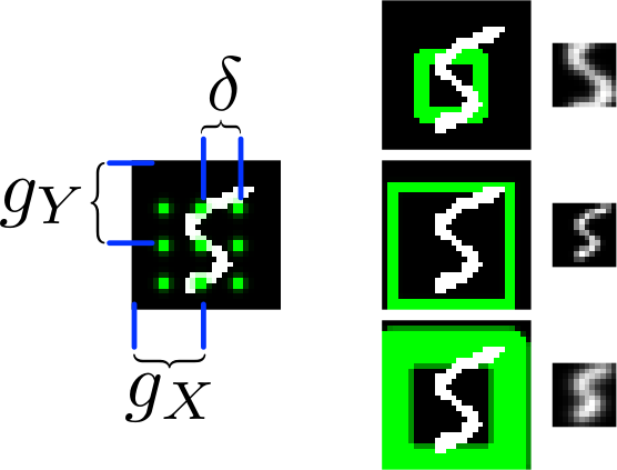
*The basic attention mechanism. (gx, gy) is the read patch center. delta is the strides. On the right: Patches with different sizes/strides and standard deviations/blurriness.*


### Results
  * Realistic looking generated images for MNIST and SVHN.
  * Structurally OK, but overall blurry images for CIFAR-10.
  * Results with attention are usually significantly better than without attention.
  * Image generation without attention starts with a blurry image and progressively sharpens it.

![DRAW SVHN Results](https://raw.githubusercontent.com/aleju/papers/master/neural-nets/images/DRAW_A_Recurrent_Neural_Network_for_Image_Generation__svhn.png?raw=true "DRAW SVHN Results")

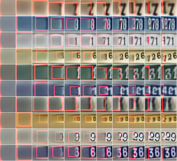
*Using DRAW with attention to generate new SVHN images.*

----------

### Rough chapter-wise notes

* 1. Introduction
  * The natural way to draw an image is in a step by step way (add some lines, then add some more, etc.).
  * Most generative neural networks however create the image in one step.
  * That removes the possibility of iterative self-correction, is hard to scale to large images and makes the image generation process dependent on a single latent distribution (input parameters).
  * The DRAW architecture generates images in multiple steps, allowing refinements/corrections.
  * DRAW is based on varational autoencoders: An encoder compresses images to codes and a decoder generates images from codes.
  * The loss function is a variational upper bound on the log-likelihood of the data.
  * DRAW uses recurrance to generate images step by step.
  * The recurrance is combined with attention via partial glimpses/foveations (i.e. the model sees only a small part of the image).
  * Attention is implemented in a differentiable way in DRAW.

* 2. The DRAW Network
  * The DRAW architecture is based on variational autoencoders:
    * Encoder: Compresses an image to latent codes, which represent the information contained in the image.
    * Decoder: Transforms the codes from the encoder to images (i.e. defines a distribution over images which is conditioned on the distribution of codes).
  * Differences to variational autoencoders:
    * Encoder and decoder are both recurrent neural networks.
    * The encoder receives the previous output of the decoder.
    * The decoder writes several times to the image array (instead of only once).
    * The encoder has an attention mechanism. It can make a decision about the read location in the input image.
    * The decoder has an attention mechanism. It can make a decision about the write location in the output image.
  * 2.1 Network architecture
    * They use LSTMs for the encoder and decoder.
    * The encoder generates a vector.
    * The decoder generates a vector.
    * The encoder receives at each time step the image and the output of the previous decoding step.
    * The hidden layer in between encoder and decoder is a distribution Q(Zt|ht^enc), which is a diagonal gaussian.
    * The mean and standard deviation of that gaussian is derived from the encoder's output vector with a linear transformation.
    * Using a gaussian instead of a bernoulli distribution enables the use of the reparameterization trick. That trick makes it straightforward to backpropagate "low variance stochastic gradients of the loss function through the latent distribution".
    * The decoder writes to an image canvas. At every timestep the vector generated by the decoder is added to that canvas.
  * 2.2 Loss function
    * The main loss function is the negative log probability: `-log D(x|ct)`, where `x` is the input image and `ct` is the final output image of the autoencoder. `D` is a bernoulli distribution if the image is binary (only 0s and 1s).
    * The model also uses a latent loss for the latent layer (between encoder and decoder). That is typical for VAEs. The loss is the KL-Divergence between Q(Zt|ht_enc) (`Zt` = latent layer, `ht_enc` = result of encoder) and a prior `P(Zt)`.
    * The full loss function is the expection value of both losses added up.
  * 2.3 Stochastic Data Generation
    * To generate images, samples can be picked from the latent layer based on a prior. These samples are then fed into the decoder. That is repeated for several timesteps until the image is finished.

* 3. Read and Write Operations
  * 3.1 Reading and writing without attention
    * Without attention, DRAW simply reads in the whole image and modifies the whole output image canvas at every timestep.
  * 3.2 Selective attention model
    * The model can decide which parts of the image to read, i.e. where to look at. These looks are called glimpses.
    * Each glimpse is defined by its center (x, y), its stride (zoom level), its gaussian variance (the higher the variance, the more blurry is the result) and a scalar multiplier (that scales the intensity of the glimpse result).
    * These parameters are calculated based on the decoder output using a linear transformation.
    * For an NxN patch/glimpse `N*N` gaussians are created and applied to the image. The center pixel of each gaussian is then used as the respective output pixel of the glimpse.
  * 3.3 Reading and writing with attention
    * Mostly the same technique from (3.2) is applied to both reading and writing.
    * The glimpse parameters are generated from the decoder output in both cases. The parameters can be different (i.e. read and write at different positions).
    * For RGB the same glimpses are applied to each channel.

* 4. Experimental results
  * They train on binary MNIST, cluttered MNIST, SVHN and CIFAR-10.
  * They then classfiy the images (cluttered MNIST) or generate new images (other datasets).
  * They say that these generated images are unique (to which degree?) and that they look realistic for MNIST and SVHN.
  * Results on CIFAR-10 are blurry.
  * They use binary crossentropy as the loss function for binary MNIST.
  * They use crossentropy as the loss function for SVHN and CIFAR-10 (color).
  * They used Adam as their optimizer.
  * 4.1 Cluttered MNIST classification
    * They classify images of cluttered MNIST. To do that, they use an LSTM that performs N read-glimpses and then classifies via a softmax layer.
    * Their model's error rate is significantly below a previous non-differentiable attention based model.
    * Performing more glimpses seems to decrease the error rate further.
  * 4.2 MNIST generation
    * They generate binary MNIST images using only the decoder.
    * DRAW without attention seems to perform similarly to previous models.
    * DRAW with attention seems to perform significantly better than previous models.
    * DRAW without attention progressively sharpens images.
    * DRAW with attention draws lines by tracing them.
  * 4.3 MNIST generation with two digits
    * They created a dataset of 60x60 images, each of them containing two random 28x28 MNIST images.
    * They then generated new images using only the decoder.
    * DRAW learned to do that.
    * Using attention, the model usually first drew one digit then the other.
  * 4.4 Street view house number generation
    * They generate SVHN images using only the decoder.
    * Results look quite realistic.
  * 4.5 Generating CIFAR images
    * They generate CIFAR-10 images using only the decoder.
    * Results follow roughly the structure of CIFAR-images, but look blurry.