#### About APAD ####
_This summer I've been Interning at an AI lab at BCM, working under
Ankit Patel in his incredible Neuroscience-meets-Deep-Learning group. 
This field is moving faster than anything else out there. Keeping intro short, 
so full post + inline pictures are on my [blog](http://rayraycano.github.io/data%20science/tech/2017/07/31/A-Paper-a-Day-GEM.html)_

## Basics ##
* __Paper__: [Gradient Episodic Memory for Continuum Learning][GED]
* __Authors__: David Lopez-Paz, Marc'Aurelio Ranzato 
* __Organizaitons__: Facebook AI Research (FAIR)
* __Topic__: Coninuum Learning
* __In One Senetence__: _Paz and Ranzato define sorely needed metrics to the
subfield of Continual Learning while developing a gradient-inspired update rule 
that avoids catastrophic forgetting_

### Background ###

Paz and Ranzato's continuum learning targets a more general problem of 
_catastrophic forgetting_, which the authors describe as "the poor ability of models to
quickly solve new problems, without forgetting previously acquired knowledge."
Recently this has been a hot topic in AI recently, as a flurry of 
papers in early summer were released discussing this topic ([Elastic Weight Consolidation][EWC],
[PathNet][PathNet], [iCaRL][iCARL], [Sluice Network][Sluice Network], [Intelligent Synapses][Intelligent Synapses]).
Avoiding catastrophic forgetting and achieving nontrivial _backwards transfer_ (BT) and _forward transfer_ (FT) are major goals for
continual learning models, and in addition, general AI. 

__Analogy Alert!__ _As Ankit explained to me originally: 
If you know how to play tennis, your experience 
*should* aid your ability to pick up ping pong (FT). 
In addition, when you return to tennis, your aptitude
in tennis shouldn't decrease (some atheletes argue that they get better
at their primary sport because they've played secondary sports, i.e. BT)._ 
 
## Paper Accomplishments ##

1. Of the 5 papers mentioned above, 0 of them formally define metrics for a
continual learner. 
2. The gradient-aligning update rule is quite clever and pretty cool.

### The Metrics ###
First, let's take a look at their formal definitions for FT and BT. 
They're displayed below. The notation is a bit confusing, so I've done my
 best to parse it.
 
[Backward And Forward Transfer LaTeX](https://www.dropbox.com/s/qrj6sxkfruj42uk/Screen%20Shot%202017-07-31%20at%204.56.05%20PM.png?dl=1)

T is the total number of tasks, enumerated from 1 to T. The bi vector is the random initialization for each task. I've omitted accuracy from this discussion because it seem too novel in the context of this paper

* Assume a fixed sequence of tasks (Numbered 1 through T)
* Forward transfer is the average accuracy of some task, task _i_, after each 
task in the sequence preceding _i_ is completed. 
    * Record the score for task _i_ upon random initialization
    * Learn task 1, record your score for task _i_. Learn task 2, record your
     score for task _i_, etc., up until task _i-1_.
    * Subtract from their score upon initialization and average these scores.
* Backwards Transfer is the average accuracy change for task _i_ after each 
task afterwards has been completed
    * Record the score for task _i_ after learning it
    * Learn task _i+1_. Now record the score for task _i_. Learn task _i+2_. Record the
    score for task _i_, etc.
    * For each score of task _i_ that recorded after completeing _i_, subtract from the first
    score for task _i_. Average these Scores

    
#### Gripes about the Metrics ####
In my opinion, these metrics don't generalize well. Continuum Learning (which I presume
is less general than _Continual_ Learning) specifies a sequence of tasks,
 meaning it is sensitive to the order of tasks. In their experiments section, 
 they use tasks that theoretically don't depend on the order in which they're learned, so in the 
 scheme of their paper this point is moot. However, Continual Learning in general
has no specification on order. Other papers concerning this topic have not discussed
task curriculums at all, while this paper glosses over it. 

__A metric I prefer: randomly sample from a pool of tasks
_n_ times. Learn these _n_ tasks in an arbitrary order. Lastly, evaluate accuracy on _i_ (for forward transfer).__ 
(This can be done over multiple trials to get a robust average)

### Gradient-Aligned Updates ###

For those new to Machine Learning, much of Deep Learning is powered by the 
[__backpropagation algorithm__][backprop]. This algorithm calculates an update that
will improve the accuracy for the problem based on an error metric. It does this by calculating what's 
called a gradient. 

__Analogy Alert!__ : _You shoot a dart at a board. You shot low by some distance __d__. 
You correct your mechanics, backwards reasoning from the missed distance, to your 
release point, and from there perhaps your throwing velocity. 
You can think of these corrections as the gradient, and the linked modification of
all the preceding components as an implementation
of the [chain rule][chainrule]. Disclaimer: 
 There is no evidence that the brain implements backpropagation_

So what does Gradient Episodic Memory (GEM) do exactly? Let's start with the Memory
part and go from there

* _Memory_: Recall those sequence of tasks we mentioned earlier? Well for each of those
tasks, let's make sure we don't forget them. We'll keep a portion of them in memory. 

* _Episodic_: Let's replay these memories to make sure we're not damaging our accuracy
on these tasks when we learn new ones. By playing them over again, we're basically going through an episode

* _Gradient_: When we look at the episode again, let's make sure the gradient doesn't
go the wrong way. What this means is: let's not unlearn what we learned on the 
previous task. 

### So How is it Done? ###

[Gradient Update Equation][Gradient Update Equation]

g is the gradient for the current task, while gk is the gradient for each previous task, calculated over the episodes in memory (Mk). The big < > notation is a dot product operator

Dot Products! In order for a gradient update to take place, they compute the dot product
of the current learning task with all the previous tasks in memory. The update is allowed
to take place if the gradient is greater than or equal to 0 for all the episodes. This translates
into constraining your update for one task to not conflict with an update for the previous task.

What if the gradient is going the wrong way? Paz and Ronzato take this gradient update
and project it to the closest possible vector that doesn't go the wrong way 
(The proof is in the pudding, eqn. 8 - 13 in the paper. It formulates the optimization as a projection
on to a cone).
 
[Gradient Update Projection Example][Gradient Update Projection Example]

 Above shows the graphical representation of the gradient update conditions, with the blue
    line being the update for the first task, while the red line is the gradient update for the current task. The right side
    shows an approximation of the optimized projection for the gradient when the dot product is negative.

### Does it work? ###
Yes. Well, kind of. 

The focus of this paper was to minimize Backwards Loss (aka
maximize Backwards Transfer). In this sense, they appear to succeed. However, 
the small improvements lack error bars, making an unconvincing case (#DLNeedsErrorBars). 
Forward Transfer is negligible on all but one experiment (there were three total).

[Results from Paper]

The plots above show performance. The right hand side demonstrates
the accuracy on the first task as the consequent tasks are learned, which each different
colored bar indicating a start to learning for a new task.

#### Knitpicking ####

* The experiments compare against Elastic Weight Consolidation (EWC). However, 
EWC was tested and optimized for Reinforcement Learning and Atari Games. I wonder
if an earnest job of optimizing EWC for the tasks at hand was done. 

* There is still no metric for parameter conservation as a result of continual/shared learning. 
A curve showing the change in accuracy across a set of tasks while increasing 
the size of the overall network would be nice. It would be interesting to compare 
all the papers on this metric. You could also evaluate the similarity of tasks
(or how well a network learns similarities in tasks) through this method.

### Summary ###
Cool Method.  Nice Paper. Less than satisfying results. But in general a
solid step forward for continual learning/overcoming catastrophic
forgetting. 


[EWC]: https://arxiv.org/pdf/1612.00796.pdf
[PathNet]: https://arxiv.org/pdf/1701.08734.pdf
[iCARL]: https://arxiv.org/pdf/1611.07725.pdf
[Sluice Network]: https://arxiv.org/pdf/1705.08142.pdf
[Intelligent Synapses]: https://openreview.net/pdf?id=rJzabxSFg
[Metrics]: https://www.dropbox.com/s/qrj6sxkfruj42uk/Screen%20Shot%202017-07-31%20at%204.56.05%20PM.png?dl=0
[Gradient]: https://www.dropbox.com/s/jye3b3mco5fs277/Screen%20Shot%202017-07-31%20at%204.55.52%20PM.png?dl=0
[Results]: https://www.dropbox.com/s/qvr95xydhtlnijw/Screen%20Shot%202017-07-31%20at%204.55.41%20PM.png?dl=0
[GED]: https://arxiv.org/pdf/1706.08840.pdf
[backprop]:https://en.wikipedia.org/wiki/Backpropagation
[chainrule]:https://en.wikipedia.org/wiki/Chain_rule
[Gradient Update Equation]:https://www.dropbox.com/s/jye3b3mco5fs277/Screen%20Shot%202017-07-31%20at%204.55.52%20PM.png?dl=1
[Gradient Update Projection Example]: https://www.dropbox.com/s/jkdkk8bmz6btl77/Screen%20Shot%202017-07-31%20at%207.36.14%20PM.png?dl=1 "Projection Update"
[Results from Paper]:https://www.dropbox.com/s/qvr95xydhtlnijw/Screen%20Shot%202017-07-31%20at%204.55.41%20PM.png?dl=1

 
 

For a traditional single-node database, the data that a transaction reads and writes is all on a single machine. For a distributed OLTP database, there are two types of transactions:

1. Local transactions are transactions that read and write data on a single machine, much like traditional transactions. A distributed database can process a local transaction as efficiently as a traditional single-node database can.
2. Distributed transactions are transactions that read and write data that is spread across multiple machines. Typically, distributed databases use two-phase commit (2PC) to commit or abort distributed transactions. Because 2PC requires multiple rounds of communications, distributed databases process distributed transactions less efficiently than local transactions.

This paper presents an alternative to 2PC, dubbed Localizing Executions via Aggressive Placement of data (LEAP), which tries to avoid the communication overheads of 2PC by aggressively moving all the data a distributed transaction reads and writes onto a single machine, effectively turning the distributed transaction into a local transaction.

#### LEAP

LEAP is based on the following assumptions and observations:

 - Transactions in an OLTP workload don't read or write many tuples.
 - Tuples in an OLTP database are typically very small.
 - Multiple transactions issued one after another may access the same data again and again.
 - As more advanced network technology becomes available (e.g. RDMA), the cost of moving data becomes smaller and smaller.

With LEAP, tuples are horizontally partitioned across a set of nodes, and each tuple is stored exactly once. Each node has two data structures:

 - a data table which stores tuples, and
 - a horizontally partitioned owner table key-value store which stores ownership information.

Consider a tuple $d = (k, v)$ with primary key $k$ and value $v$. The owner table contains an entry $(k, o)$ indicating that node o owns the tuple with key $k$. The node $o$ contains a $(k, v)$ entry in its data table. The owner table key-value store is partitioned across nodes using any arbitrary partitioning scheme (e.g. hash-based, range-based).

When a node initiates a transaction, it requests ownership of every tuple it reads and writes. This migrates the tuples to the initiating node and updates the ownership information to reflect the ownership transfer. Here's how the ownership transfer protocol works. For a given tuple $d = (k, v)$, the requester is the node requesting ownership of $d$, the partitioner is the node with ownership information $(k, o)$, and the owner is the node that stores $d$.

 - First, the requester sends an owner request with key k to the partitioner.
 - Then, the partitioner looks up the owner of the tuple with k in its owner table and sends a transfer request to the owner.
 - The owner retrieves the value of the tuple and sends it in a transfer response back to the requester. It also deletes its copy of the tuple.
 - Finally, the requester sends an inform message to the partitioner informing it that the ownership transfer was complete. The partitioner updates its owner table to reflect the new owner.

Also note that

 - if the requester, partitioner, and owner are all different nodes, then this scheme requires 4 messages,
 - if the partitioner and owner are the same, then this scheme requires 3 messages, and
 - if the requester and partitioner are the same, then this scheme requires 2 messages.

If the transfer request is dropped and the owner deletes the tuple, data is lost. See the appendix for information on how to make this ownership transfer fault tolerant. Also see the paper for a theoretical comparison of 2PC and LEAP.

#### LEAP-Based OLTP Engine

L-Store is a distributed OLTP database based on H-Store which uses LEAP to manage transactions. Transactions acquire read/write locks on individual tuples and use strict two-phase locking. Transactions are assigned globally unique identifiers, and deadlock prevention is implemented with a wait-die scheme where lower timestamped transactions have higher priority. That is, higher priority threads wait on lower priority threads, but lower priority threads abort rather than wait on higher priority threads.

Concurrent local transactions are processed as usual; what's interesting is concurrent transfer requests. Imagine a transaction is requesting ownership of a tuple on another node.

 - First, the requester creates a request lock locally indicating that it is currently trying to request ownership of the tuple. It then sends an owner request to the partitioner.
 - The partitioner may receive multiple concurrent owner requests. It processes them serially using the wait-die scheme. As an optimization, it processes requests in decreasing timestamp order to avoid aborts whenever possible. It then forwards a transfer request to the owner.
 - If the owner is currently accessing the tuple being requested, it again uses a wait-die scheme to access the tuple before sending it back to the owner.
 - Finally, the owner changes the request lock into a normal data lock and continues processing.

If a transaction cannot successfully get ownership of a tuple, it aborts. L-Store also uses logging and checkpointing for fault tolerance (see paper for details).

One problem of training deep networks is that the features of lower-layer networks change while the upper-layer networks have already been adjusted to the previous lower-layer features. The phenomenon of changing inputs while optimizing is called *internal covariate shift*.

Batch normalization is done at training time for each mini batch.

## Ideas

* Training converges faster, if input is whitened (zero means, unit variances, decorrelated).
* Normalization parameters have to be computed within the gradient calculation step to prevent the model from blowing up

## What Batch Normalization is

For a layer with $d$-dimensional input $x = (x^{(1)}, \dots, x^{(d)})$, we will normalize
each dimension 
$$\hat{x}^{(k)} = \frac{x^{(k)} - \mathbb{E}[x^{(k)}]}{\sqrt{Var[x^{(k)}]}}$$
where the expectation and the variance are computed over the training data set. This does *not* decorrelate the features, though.

Additionally, for each activation $x^{(k)}$ two paramters $\gamma^{(k)}, \beta^{(k)}$ are introduced which scale and shift the feature:

$$y^{(k)} = \gamma^{(k)} \cdot \hat{x}^{(k)} + \beta^{(k)}$$

Those two parameters (per feature) are learnable!

## Effect of Batch normalization

* Higher learning rates can be used
* Initialization is less important
* Acts as a regularizer, eliminating the need for dropout in some cases
* Faster training

## Datasets

* reaching 4.9% top-5 validation error (and 4.8% test error) on ImageNet classification

## Used by

* [Going Deeper with Convolutions](http://www.shortscience.org/paper?bibtexKey=journals/corr/SzegedyLJSRAEVR14)
* [Deep Residual Learning for Image Recognition](http://www.shortscience.org/paper?bibtexKey=journals/corr/HeZRS15#martinthoma)

## See also

* [other summaries](http://www.shortscience.org/paper?bibtexKey=conf/icml/IoffeS15)

  * They describe a model to locate faces in images.
  * Their model uses information from suspected face regions *and* from the corresponding suspected body regions to classify whether a region contains a face.
  * The intuition is, that seeing the region around the face (specifically where the body should be) can help in estimating whether a suspected face is really a face (e.g. it might also be part of a painting, statue or doll).

### How
  * Their whole model is called "CMS-RCNN" (Contextual Multi-Scale Region-CNN).
  * It is based on the "Faster R-CNN" architecture.
  * It uses the VGG network.
  * Subparts of their model are: MS-RPN, CMS-CNN.
  * MS-RPN finds candidate face regions. CMS-CNN refines their bounding boxes and classifies them (face / not face).
  * **MS-RPN** (Multi-Scale Region Proposal Network)
    * "Looks" at the feature maps of the network (VGG) at multiple scales (i.e. before/after pooling layers) and suggests regions for possible faces.
    * Steps:
      * Feed an image through the VGG network.
      * Extract the feature maps of the three last convolutions that are before a pooling layer.
      * Pool these feature maps so that they have the same heights and widths.
      * Apply L2 normalization to each feature map so that they all have the same scale.
      * Apply a 1x1 convolution to merge them to one feature map.
      * Regress face bounding boxes from that feature map according to the Faster R-CNN technique.
  * **CMS-CNN** (Contextual Multi-Scale CNN):
    * "Looks" at feature maps of face candidates found by MS-RPN and classifies whether these regions contains faces.
    * It also uses the same multi-scale technique (i.e. take feature maps from convs before pooling layers).
    * It uses some area around these face regions as additional information (suspected regions of bodies).
    * Steps:
      * Receive face candidate regions from MS-RPN.
      * Do per candidate region:
        * Calculate the suspected coordinates of the body (only based on the x/y-position and size of the face region, i.e. not learned).
        * Extract the feature maps of the *face* region (at multiple scales) and apply RoI-Pooling to it (i.e. convert to a fixed height and width).
        * Extract the feature maps of the *body* region (at multiple scales) and apply RoI-Pooling to it (i.e. convert to a fixed height and width).
        * L2-normalize each feature map.
        * Concatenate the (RoI-pooled and normalized) feature maps of the face (at multiple scales) with each other (creates one tensor).
        * Concatenate the (RoI-pooled and normalized) feature maps of the body (at multiple scales) with each other (creates another tensor).
        * Apply a 1x1 convolution to the face tensor.
        * Apply a 1x1 convolution to the body tensor.
        * Apply two fully connected layers to the face tensor, creating a vector.
        * Apply two fully connected layers to the body tensor, creating a vector.
        * Concatenate both vectors.
        * Based on that vector, make a classification of whether it is really a face.
        * Based on that vector, make a regression of the face's final bounding box coordinates and dimensions.
  * Note: They use in both networks the multi-scale approach in order to be able to find small or tiny faces. Otherwise, after pooling these small faces would be hard or impossible to detect.

### Results
  * Adding context to the classification (i.e. the body regions) empirically improves the results.
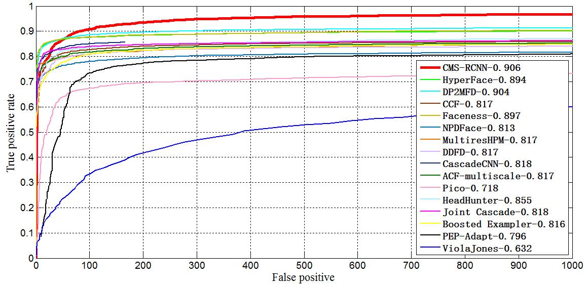
  * Their model achieves the highest recall rate on FDDB compared to other models. However, it has lower recall if only very few false positives are accepted.
  * FDDB ROC curves (theirs is bold red):
    * ![FDDB results](https://raw.githubusercontent.com/aleju/papers/master/neural-nets/images/CMS-RCNN__fddb.jpg?raw=true "FDDB results")
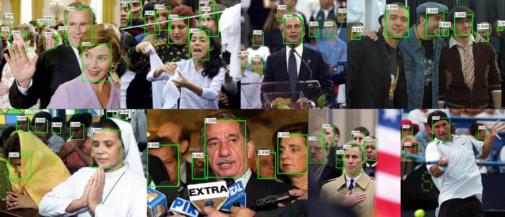
  * Example results on FDDB:
    * ![FDDB examples](https://raw.githubusercontent.com/aleju/papers/master/neural-nets/images/CMS-RCNN__examples.jpg?raw=true "FDDB examples")

https://www.youtube.com/watch?v=vQk_Sfl7kSc&feature=youtu.be

  * The paper describes a method to transfer the style (e.g. choice of colors, structure of brush strokes) of an image to a whole video.
  * The method is designed so that the transfered style is consistent over many frames.
  * Examples for such consistency:
    * No flickering of style between frames. So the next frame has always roughly the same style in the same locations.
    * No artefacts at the boundaries of objects, even if they are moving.
    * If an area gets occluded and then unoccluded a few frames later, the style of that area is still the same as before the occlusion.

### How
  * Assume that we have a frame to stylize $x$ and an image from which to extract the style $a$.
  * The basic process is the same as in the original Artistic Style Transfer paper, they just add a bit on top of that.
  * They start with a gaussian noise image $x'$ and change it gradually so that a loss function gets minimized.
  * The loss function has the following components:
    * Content loss *(old, same as in the Artistic Style Transfer paper)*
      * This loss makes sure that the content in the generated/stylized image still matches the content of the original image.
      * $x$ and $x'$ are fed forward through a pretrained network (VGG in their case).
      * Then the generated representations of the intermediate layers of the network are extracted/read.
      * One or more layers are picked and the difference between those layers for $x$ and $x'$ is measured via a MSE.
      * E.g. if we used only the representations of the layer conv5 then we would get something like `(conv5(x) - conv5(x'))^2` per example. (Where conv5() also executes all previous layers.)
    * Style loss *(old)*
      * This loss makes sure that the style of the generated/stylized image matches the style source $a$.
      * $x'$ and $a$ are fed forward through a pretrained network (VGG in their case).
      * Then the generated representations of the intermediate layers of the network are extracted/read.
      * One or more layers are picked and the Gram Matrices of those layers are calculated.
      * Then the difference between those matrices is measured via a MSE.
    * Temporal loss *(new)*
      * This loss enforces consistency in style between a pair of frames.
      * The main sources of inconsistency are boundaries of moving objects and areas that get unonccluded.
      * They use the optical flow to detect motion.
        * Applying an optical flow method to two frames $(i, i+1)$ returns per pixel the movement of that pixel, i.e. if the pixel at $(x=1, y=2)$ moved to $(x=2, y=4)$ the optical flow at that pixel would be $(u=1, v=2)$.
        * The optical flow can be split into the forward flow (here `fw`) and the backward flow (here `bw`). The forward flow is the flow from frame i to i+1 (as described in the previous point). The backward flow is the flow from frame $i+1$ to $i$ (reverse direction in time).
      * Boundaries
        * At boundaries of objects the derivative of the flow is high, i.e. the flow "suddenly" changes significantly from one pixel to the other.
        * So to detect boundaries they use (per pixel) roughly the equation `gradient(u)^2 + gradient(v)^2 > length((u,v))`.
      * Occlusions and disocclusions
        * If a pixel does not get occluded/disoccluded between frames, the optical flow method should be able to correctly estimate the motion of that pixel between the frames. The forward and backward flows then should be roughly equal, just in opposing directions.
        * If a pixel does get occluded/disoccluded between frames, it will not be visible in one the two frames and therefore the optical flow method cannot reliably estimate the motion for that pixel. It is then expected that the forward and backward flow are unequal.
        * To measure that effect they roughly use (per pixel) a formula matching `length(fw + bw)^2 > length(fw)^2 + length(bw)^2`.
      * Mask $c$
        * They create a mask $c$ with the size of the frame.
        * For every pixel they estimate whether the boundary-equation *or* the disocclusion-equation is true.
        * If either of them is true, they add a 0 to the mask, otherwise a 1. So the mask is 1 wherever there is *no* disocclusion or motion boundary.
      * Combination
        * The final temporal loss is the mean (over all pixels) of $c*(x-w)^2$.
          * $x$ is the frame to stylize.
          * $w$ is the previous *stylized* frame (frame i-1), warped according to the optical flow between frame i-1 and i.
          * `c` is the mask value at the pixel.
        * By using the difference `x-w` they ensure that the difference in styles between two frames is low.
        * By adding `c` they ensure the style-consistency only at pixels that probably should have a consistent style.
    * Long-term loss *(new)*
      * This loss enforces consistency in style between pairs of frames that are longer apart from each other.
      * It is a simple extension of the temporal (short-term) loss.
      * The temporal loss was computed for frames (i-1, i). The long-term loss is the sum of the temporal losses for the frame pairs {(i-4,i), (i-2,i), (i-1,i)}.
      * The $c$ mask is recomputed for every pair and 1 if there are no boundaries/disocclusions detected, but only if there is not a 1 for the same pixel in a later mask. The additional condition is intended to associate pixels with their closest neighbours in time to minimize possible errors.
      * Note that the long-term loss can completely replace the temporal loss as the latter one is contained in the former one.
  * Multi-pass approach *(new)*
    * They had problems with contrast around the boundaries of the frames.
    * To combat that, they use a multi-pass method in which they seem to calculate the optical flow in multiple forward and backward passes? (Not very clear here what they do and why it would help.)
  * Initialization with previous frame *(new)*
    * Instead of starting at a gaussian noise image every time, they instead use the previous stylized frame.
    * That immediately leads to more similarity between the frames.